Federal elections results by poll section part 2 : map census data to poll section and plot the results
This Notebook builds on the poll_final sf dataframe we built in the first part of this project. poll_final contains the poll results by party and the geometry for each poll for the 2015 Federal Elections of 2015.
We will use the cancensus package to download sociodemographic data and geometry from the 2016 Canadian Census. We will then “dispatch” the population characteristics to each poll sections and plot the relationship between education and the results of the three main parties (libéral, conservateur and ndp).
This notebook uses the tidyverse for wranling and plotting data, the cancensus package to download the Canadian Census data, the lwgeom package for making polygons “valid” and the `sf package for finding their intersections.
Disclaimer: I am not a poticial science expert, I just like messing around with data when my kids wake me up at night. The results here may be common knowledge already, my assumptions may be extremely wrong and my code could just be bugged.
Code
As usual, the code for this post is available on my GitHub repo and is then hosted on my Hugo blog generated by blogdown and hosted on github/netlify.
Functions
I created three functions that wrap around the cancensus package:
get_cancensus_pct takes a parent vector and a generation level (first or last) for
the children vectors and return a dataframe showing the percentage each child vectors represents
at the geographic level specified.
get_cancensus_labels takes a parent vector and a generation level (first or last) for
the children vectors and return the labels for the parent and children vectors.
get_cancensus_data build on these two functions. It takes a vector of parent
vectors names and a generation level and returns a list of three objectS:
- a dataframe with the percentages
- a dictionnary showing which child are contained in each parent vector
- a list of the parent vectors.
Finally, the wrapper function automatically adds line changes to
strings after a certain length, allowing titles to fit inside ggplot.
I borrowed it from the internet a while ago.
Code snippets I will be coming back to this script for
- My three cancensus functions.
- example of st_make_valid() and st_intersection()
- combining purrr and ggplot using map2(data,..)
- usethis::edit_r_profile() , then add the following for cancensus:
- options(cancensus.api_key = Sys.getenv(“cancensus_api”))
- options(cancensus.cache_path = ‘C:/MY_CACHE_PATH’)
- options(cancensus.api_key = Sys.getenv(“cancensus_api”))
Getting the census data and applying it to the poll sections
Getting the census data and shapefile is pretty straightforward when done using the cancensus package. “v_CA16_5051” is the highest level of schooling.
We download the census data at the Dissemination Area (DA) level, which is the smallest geographical level for which Statistics Canada will release data. Its population is between 400-700 persons.
Once we have the DA data, we find the intersection between the DA and the poll sections.
Lines that should be identical in both files are not always 100% accurate, which leads to small intersection between polygons that should not intersect. To prevent this,
I ignore intersections that represent less than 10% of either the DA or poll polygon.
We then distribute the DA population to the polls. We make three important assumptions:
- elector population is proportional to total populattion (we should use population aged 18+ at the very least)
- DA population is uniformly distributed on the whole area
- Participation rate is equal among all DA that touch a poll
To make analysis easier, we group the highest levels of schooling in three groups:
- No high school diploma
- High school, college, trade or university certificate below bachelor
- University (bachelor degree or above)
Results
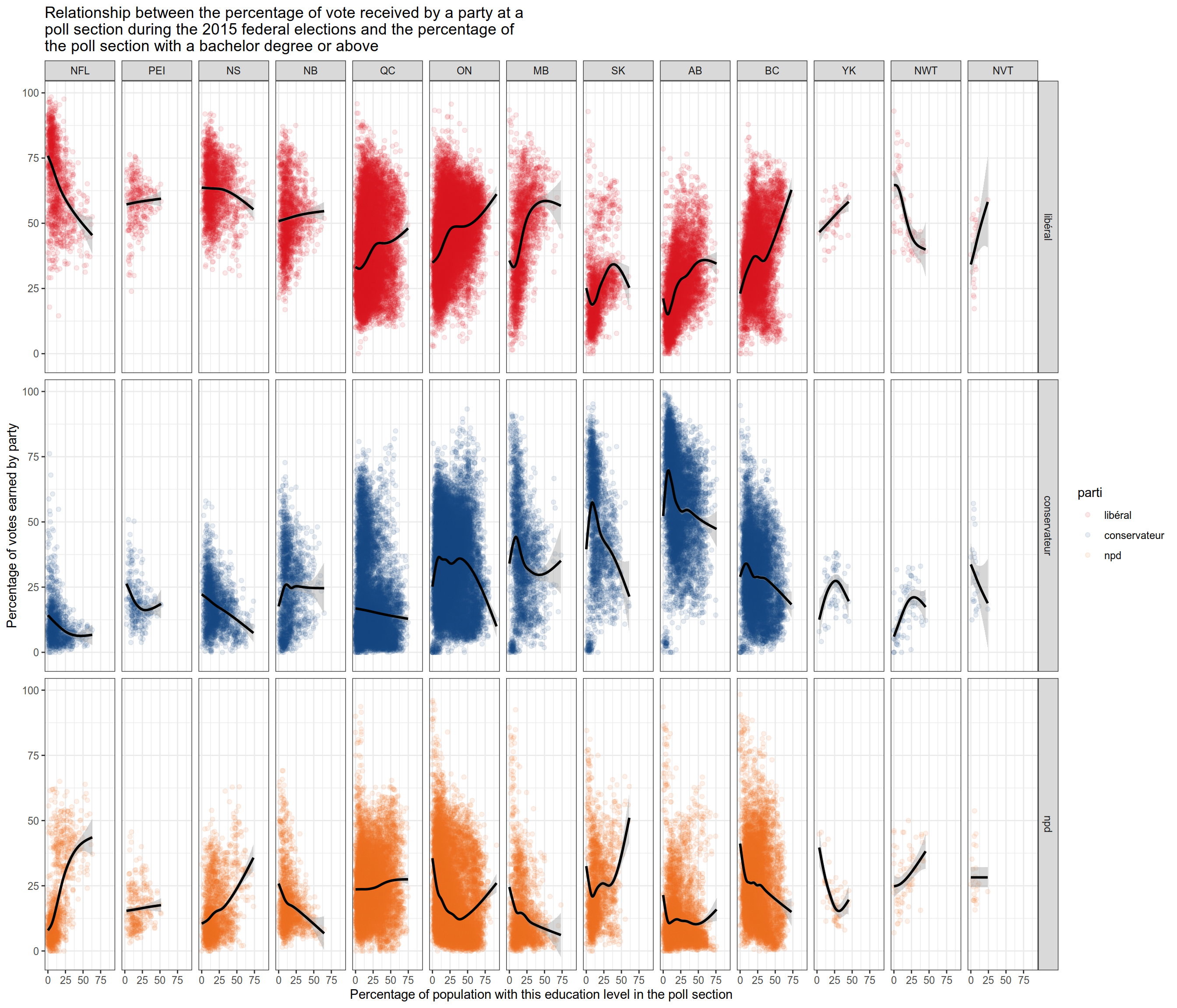
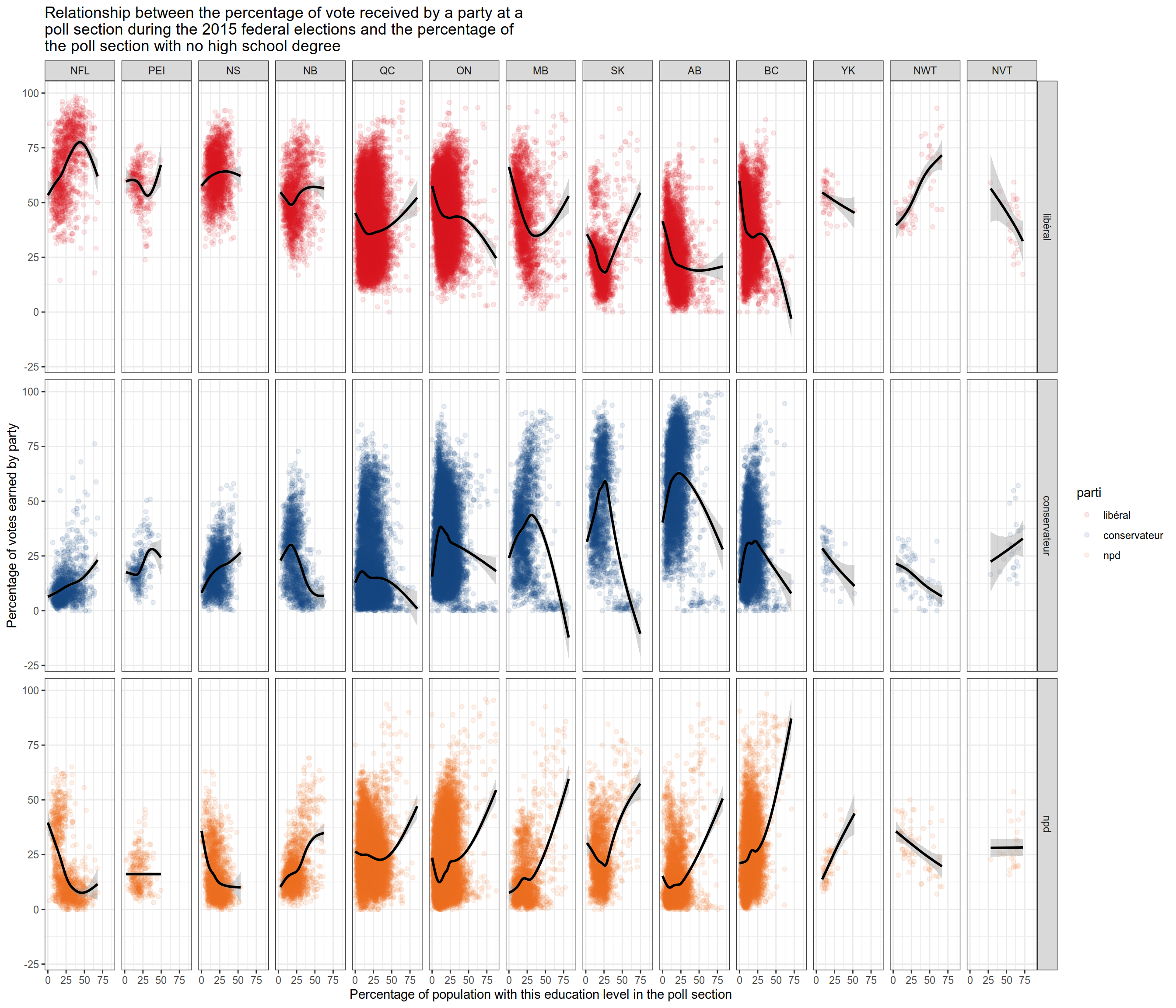
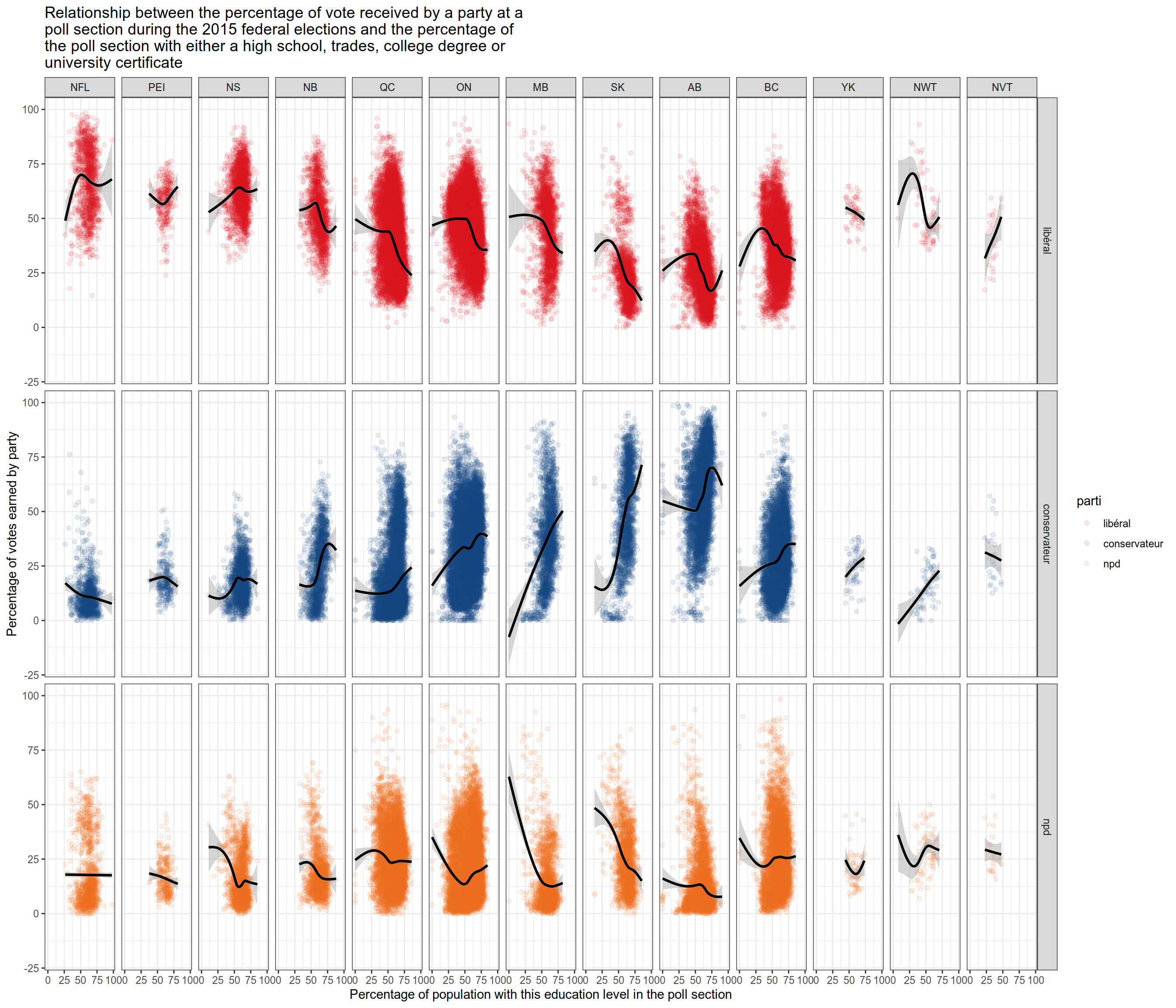
Finally, we make scatter plots showing the relationship between the level of schooling of the poll and the results of the three main parties. Each dot represents one polling station. I have broken down the poll between the 10 provinces and the 3 territories to see if the trends hold between different areas.
Province codes:
- 10 Newfoundland and Labrador
- 11 Prince Edward Island
- 12 Nova Scotia
- 13 New Brunswick
- 24 Quebec
- 35 Ontario
- 46 Manitoba
- 47 Saskatchewan
- 48 Alberta
- 59 British Columbia
- 60 Yukon
- 61 Northwest Territories
- 62 Nunavut
Results are not uniform across provinces, but I spotted the following trends outside of the Atlantic provinces (NFL, PEI, NS and NB).
A high share of population with no high school will help the NPD in most provinces outside of the Atlantic.
The conservative party appears to thrive in poll sections with a high proportion of “middle level” education such as high school or college degrees, trade certificates outside of the Atlantic.
A high share of university degrees typically helps the Libéral, except in the Atlantic, where it will favour the NPD. It never helps the conservative party.