
Mapping UN Votes on a hex grid
EDIT 2019: hexmapr has been renamed to geogrid. Also calculate_cell_size() has been deprecated to become calculate_grid()
Today, David Robinson (@drob) tweeted about his unvotes package which contains the history of the United Nations General Assembly voting :
Check out my unvotes package, with history of United Nations General Assembly voting: https://t.co/VDQ3kGMQtf
— David Robinson (@drob) January 9, 2018
To me, this dataset just screams to be mapped. Especially on a hex map, as I have been
looking for an excuse to try Joseph Bailey’s (@iammrbailey) hexmapr package
since I saw this tweet two months ago:
My 1st R package! https://t.co/dI3GJbC7FQ Automatically turn geospatial polygons like states into regular/hexagonal grids #rstats #ggplot2 pic.twitter.com/dxvYCZWJzU
— Joseph Bailey (@iammrbailey) October 31, 2017
Hex map arrange the polygons of the countries on a grid of hexagons, where each country has the same size, which is great since each vote has the same value and huge countries such as Canada or Russia see their visual importance exagerated.
In this post, we will first map the results from the most recent important UN vote on a leaflet using Andy South (@southmapr)’s rworldmap package as a source for the world map shapefile.
Then we will attempt to convert the world map to a hex map using the hexmapr package and map the result using ggplot.
Get the votes and map them on the world map
#devtools::install_github("sassalley/hexmapr")
#install.packages("geogrid")
library(plyr)
library(dplyr)
library(unvotes)
library(rworldmap)
library(leaflet)
library(viridis)
library(geogrid)
library(leaflet)
library(ggplot2)
library(gridExtra)
library(sf)
library(widgetframe) # for inserting datatables and leaflets inside the blog
lastvote <- un_votes %>%
  inner_join(un_roll_calls, by = "rcid") %>%
  filter(importantvote == 1) %>%
  filter(date == max(date))
# save title of the last vote for use in the legend
lastvote_desc <- lastvote %>% distinct(descr) %>% pull(descr)
# attach votes to shapefile from rworldmap using ISO alpha2 country code
# drop the polygons for which there has never been a vote using inner_join
sf <- st_as_sf(rworldmap::countriesCoarseLessIslands)  %>%
  select(NAME,ISO_A2) %>%
  left_join(lastvote %>% select(ISO_A2 = country_code, vote)) %>%
  inner_join(un_votes %>%
               distinct(country_code) %>%
               select(ISO_A2 = country_code))
# create a palette
ndistinct<- as.numeric(lastvote %>%
                         summarise( count = n_distinct(vote)) %>%
                         select(count))
mypal <- leaflet::colorFactor(viridis_pal(option="C")(ndistinct),
                              domain = lastvote$vote, reverse = TRUE)
# map votes using leaflet
leaflet(sf) %>%
  addProviderTiles(providers$Stamen.TonerLines) %>%
  addProviderTiles(providers$Stamen.TonerLabels) %>%
  addPolygons( fillColor = ~mypal(vote),
               color = "none",
               label = ~ paste0(NAME, " - ", vote )) %>%
  addLegend("bottomleft",
            pal = mypal,
            values = ~ vote,
            title = ~ paste0("votes on ", lastvote_desc))  %>%
  widgetframe::frameWidget(., width = '95%')
Convert the world map to a hex grid and map the votes
Here, we follow the hexmapr vignette, except that we use the
as(sf, 'Spatial') function instead of read_polygons() since we dont have
an actual shapefile to read. The documentation of read_polygons() states that it
is “basically st_read”, and it seems to work.
original_shapes <- as(sf, 'Spatial')
#original_details <-get_shape_details(original_shapes)
raw <- as(sf, 'Spatial')
raw@data$xcentroid <- coordinates(raw)[,1]
raw@data$ycentroid <- coordinates(raw)[,2]
clean <- function(shape){
  shape@data$id = rownames(shape@data)
  shape.points = fortify(shape, region="id")
  shape.df = join(shape.points, shape@data, by="id")
}
result_df_raw <- clean(raw)
rawplot <- ggplot(result_df_raw) +
  geom_polygon( aes(x=long, y=lat, fill = vote, group = group)) +
  geom_text(aes(xcentroid, ycentroid, label = substr(NAME,1,4)),
            size=2,color = "white") +
  coord_equal() +
  scale_fill_viridis(discrete = T) +
  guides(fill=FALSE) +
  theme_void()
#new_cells_hex <-  calculate_cell_size(original_shapes, original_details,0.03, 'hexagonal', 6)
new_cells_hex <-  calculate_grid(original_shapes, 0.03, 'hexagonal', 6)
resulthex <- assign_polygons(original_shapes,new_cells_hex)
result_df_hex <- clean(resulthex)
hexplot <- ggplot(result_df_hex) +
  geom_polygon( aes(x=long, y=lat, fill = vote, group = group)) +
  geom_text(aes(V1, V2, label = substr(NAME,1,4)), size=2,color = "white") +
  scale_fill_viridis(discrete=T) +
  coord_equal() +
  guides(fill=FALSE) +
  theme_void()
gridExtra::grid.arrange(rawplot,hexplot, layout_matrix = rbind(c(1,1), c(2,2)))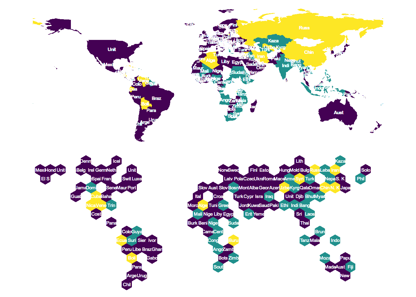
Conclusion
It sorta “worked”! We achieved our goal to convert the world map to a hex grid show the votes, which was our initial goal.
I have to admit that I am a bit disappointed with the resulting grid map.
I believe the algorithm focussed too much on recreating a map that had roughly
the same shape as the original at the expense of keeping countries on their home
continent. As a consequence, a huge “North America” block was created
using countries from Europe (United Kingdown, Luxembourg, etc..) and Africa
(Senegal, Mauritania, etc..).
I believe that the hex grid still allows us to see more easily that the vote was mostly a yes (purple), while the world map would lead us to believe that most of Asia voted no, because of Russia and China.
This might be a case of where a well-designed table would have done a better job, depending on the message that we want to convey.
Maybe an option to create groups (continents) and force countries in these groups to stick together would make finding a country on the hex map easier.
Huge thanks to the package developers.