
Bayesian optimization of xgboost hyperparameters for a Poisson regression in R
UPDATE 2020: skimr v2 now produces nice html in rmarkdown, so skimr::kable() has been deprecated. https://www.r-bloggers.com/reintroducing-skimr-v2-a-year-in-the-life-of-an-open-source-r-project/
Introduction
Ratemaking models in insurance routinely use Poisson regression to model the frequency of auto insurance claims. They usually are GLMs but some insurers are moving towards GBMs, such as xgboost.
xgboosthas multiple hyperparameters that can be tuned to obtain a better predictive power. There are multiple ways to tune these hyperparameters. In order of efficiency are the grid search, the random search and the bayesian optimization search.
In this post, we will compare the results of xgboost hyperparameters for a Poisson regression in R using a random search versus a bayesian search. Two packages wills be compared for the bayesian approach: the mlrMBO package and the rBayesianOptimization package.
We will model the number of auto insurance claims based on characteristics of the car and driver, while offsetting for exposure. The data comes from the insuranceData package.
For most model types, mlrMBO can be used in combination with the mlr package to find the best hyperparameters directly. As far as I know the mlr package doesnt handle poisson regression, so we will have to create our own function to maximise.
I tried the rBayesianOptimization package after being inspired by this post from Max Kuhn from 2016. I do not recommend using this package because it sometimes recycles hyperparameters and hasnt been updated on github since 2016.
Keep your eyes peeled: Max Kuhn (@topepos) said that tidymodels might do this in the first half of 2019.
library(xgboost)
library(insuranceData) # example dataset https://cran.r-project.org/web/packages/insuranceData/insuranceData.pdf
library(tidyverse) # for data wrangling
library(rBayesianOptimization) # to create cv folds and for bayesian optimisation
library(mlrMBO)  # for bayesian optimisation
library(skimr) # for summarising databases
library(purrr) # to evaluate the loglikelihood of each parameter set in the random grid search
require("DiceKriging") # mlrmbo requires this
require("rgenoud") # mlrmbo requires this

switch_generate_interim_data <- FALSE
Preparing the data
First, we load the dataCar data from the insuranceData package. It contains 67 856 one-year vehicle insurance policies taken out in 2004 or 2005.
The dependent variable is numclaims, which represents the number of claims.
The exposure variable represents the “number of year of exposure” and is used as the offset variable. It is bounded between 0 and 1.
Finally, the independent variables are as follow:
veh_value, the vehicle value in tens of thousand of dollars,
veh_body, y vehicle body, coded as BUS CONVT COUPE HBACK HDTOP MCARA MIBUS PANVN RDSTR SEDAN STNWG TRUCK UTE,
veh_age, 1 (youngest), 2, 3, 4,
gender, a factor with levels F M,
areaa factor with levels A B C D E F,
agecat1 (youngest), 2, 3, 4, 5, 6
# load insurance data
data(dataCar)
mydb <- dataCar %>% select(numclaims, exposure, veh_value, veh_body,
                           veh_age, gender, area, agecat)
label_var <- "numclaims"
offset_var <- "exposure"
feature_vars <- mydb %>%
  select(-one_of(c(label_var, offset_var))) %>%
  colnames()

#skimr::skim(mydb ) %>%
  #skimr::kable() #
  # update 2020 : Now, calling skim(), within an RMarkdown doc should produce something
  # nice by default.
  #
  # skim(chickwts)
  #
  # Data summary Name   chickwts
  # Number of rows  71
  # Number of columns   2
  # _______________________
  # Column type frequency:
# factor    1
# numeric   1
# ________________________
# Group variables   None
#
# Variable type: factor
# skim_variable     n_missing   complete_rate   ordered     n_unique    top_counts
# feed  0   1   FALSE   6   soy: 14, cas: 12, lin: 12, sun: 12
#
# Variable type: numeric
# skim_variable     n_missing   complete_rate   mean    sd  p0  p25     p50     p75     p100    hist
# weight    0   1   261.31  78.07   108     204.5   258     323.5   423     ▆▆▇▇▃
#
# You get a nice html version of both the summary header and the skimr subtables
# for each type of data.
#
# In this context, you configure the output the same way you handle other knitr
# code chunks.
#
# This means that we’re dropping direct support for kable.skim_df() and
# pander.skim_df(). But you can still get pretty similar results to these
Insurance ratemaking often requires monotonous relationships. In our case, we will arbitrarily force the number of claims to be non-increasing with the age of the vehicle.
The code below imports the data, one-hot encodes dummy variables, converts the data frame to a xgb.DMatrix for xgboost consumption, sets the offset for exposure, sets the constraints and defines the 3 folds we will use for cross-validation.
# one hot encoding of categorical (factor) data
myformula <- paste0( "~", paste0( feature_vars, collapse = " + ") ) %>%
  as.formula()

dummyFier <- caret::dummyVars(myformula, data=mydb, fullRank = TRUE)
dummyVars.df <- predict(dummyFier,newdata = mydb)
mydb_dummy <- cbind(mydb %>% select(one_of(c(label_var, offset_var))),
                    dummyVars.df)
rm(myformula, dummyFier, dummyVars.df)

# get  list the column names of the db with the dummy variables
feature_vars_dummy <-  mydb_dummy  %>%
  select(-one_of(c(label_var, offset_var))) %>%
  colnames()

# create xgb.matrix for xgboost consumption
mydb_xgbmatrix <- xgb.DMatrix(
  data = mydb_dummy %>% select(feature_vars_dummy) %>% as.matrix,
  label = mydb_dummy %>% pull(label_var),
  missing = "NAN")

#base_margin: apply exposure offset
setinfo(mydb_xgbmatrix,"base_margin",
        mydb %>% pull(offset_var) %>% log() )
## [1] TRUE# a fake constraint, just to show how it is done.
#Here we force "the older the car, the less likely are claims"
myConstraint <- data_frame(Variable = feature_vars_dummy) %>%
mutate(sens = ifelse(Variable == "veh_age", -1, 0))
# random folds for xgb.cv
cv_folds = rBayesianOptimization::KFold(mydb_dummy$numclaims,
nfolds= 3,
stratified = TRUE,
seed= 0)Example 1: Optimize hyperparameters using a random search (non bayesian)
We will start with a quick example of random search.
I don’t use caret for the random search because it has a hard time with poisson regression.
First, we generate 20 random sets of hyperparameters. I will force gamma = 0 for half the sets.I will also hardcode an extra set of parameters named simon_params because I find this combination is often a good starting point.
# generate hard coded parameters
simon_params <- data.frame(max_depth = 6,
                           colsample_bytree= 0.8,
                           subsample = 0.8,
                           min_child_weight = 3,
                           eta  = 0.01,
                           gamma = 0,
                           nrounds = 200) %>%
  as_tibble()
# generate 20 random models
how_many_models <- 20
max_depth <-        data.frame(max_depth = floor(runif(how_many_models)*5 ) + 3)  # 1 à 4
colsample_bytree <- data.frame(colsample_bytree =runif(how_many_models) * 0.8 + 0.2)  # 0.2 à 1
subsample <-        data.frame(subsample =runif(how_many_models) * 0.8 + 0.2) # 0.2 à 1
min_child_weight <- data.frame(min_child_weight = floor(runif(how_many_models) * 10) + 1) # 1 à 10
eta <-              data.frame(eta = runif(how_many_models) * 0.06 + 0.002) # 0.002 à 0.062
gamma <-            data.frame(gamma =c(rep(0,how_many_models/2), runif(how_many_models/2)*10)) # 0 à 10
nrounds <-          data.frame(nrounds = rep(2e2,how_many_models)) # max 200

random_grid <-max_depth %>%
  bind_cols(colsample_bytree ) %>%
  bind_cols(subsample) %>%
  bind_cols(min_child_weight) %>%
  bind_cols(eta) %>%
  bind_cols(gamma) %>%
  bind_cols(nrounds)  %>% as_tibble()
# combine random and hardcoded parameters
df.params <- simon_params %>%  bind_rows(random_grid) %>%
  mutate(rownum = row_number(),
         rownumber = row_number())
list_of_param_sets <- df.params %>% nest(-rownum)
Here are the hyperparameters that will be tested:
knitr::kable(df.params)| max_depth | colsample_bytree | subsample | min_child_weight | eta | gamma | nrounds | rownum | rownumber |
|---|---|---|---|---|---|---|---|---|
| 6 | 0.8000000 | 0.8000000 | 3 | 0.0100000 | 0.000000 | 200 | 1 | 1 |
| 4 | 0.3697140 | 0.7176482 | 3 | 0.0447509 | 0.000000 | 200 | 2 | 2 |
| 5 | 0.7213390 | 0.8263462 | 5 | 0.0259997 | 0.000000 | 200 | 3 | 3 |
| 7 | 0.3004441 | 0.6424290 | 4 | 0.0215211 | 0.000000 | 200 | 4 | 4 |
| 4 | 0.4137765 | 0.6237757 | 7 | 0.0474252 | 0.000000 | 200 | 5 | 5 |
| 7 | 0.5088913 | 0.8314850 | 3 | 0.0141615 | 0.000000 | 200 | 6 | 6 |
| 7 | 0.2107123 | 0.2186650 | 5 | 0.0446673 | 0.000000 | 200 | 7 | 7 |
| 6 | 0.5059104 | 0.5817841 | 8 | 0.0093015 | 0.000000 | 200 | 8 | 8 |
| 6 | 0.8957527 | 0.7858510 | 1 | 0.0167293 | 0.000000 | 200 | 9 | 9 |
| 3 | 0.4722792 | 0.7541852 | 9 | 0.0105983 | 0.000000 | 200 | 10 | 10 |
| 4 | 0.5856641 | 0.5820957 | 4 | 0.0163778 | 0.000000 | 200 | 11 | 11 |
| 3 | 0.6796527 | 0.8889676 | 9 | 0.0055361 | 3.531973 | 200 | 12 | 12 |
| 6 | 0.5948330 | 0.5504777 | 4 | 0.0405373 | 2.702602 | 200 | 13 | 13 |
| 4 | 0.3489741 | 0.3958378 | 4 | 0.0545762 | 9.926841 | 200 | 14 | 14 |
| 6 | 0.8618987 | 0.2565432 | 5 | 0.0487349 | 6.334933 | 200 | 15 | 15 |
| 5 | 0.7347734 | 0.2795729 | 9 | 0.0498385 | 2.132081 | 200 | 16 | 16 |
| 6 | 0.8353919 | 0.4530174 | 9 | 0.0293165 | 1.293724 | 200 | 17 | 17 |
| 7 | 0.2863549 | 0.6149074 | 4 | 0.0266050 | 4.781180 | 200 | 18 | 18 |
| 4 | 0.7789688 | 0.7296041 | 8 | 0.0506522 | 9.240745 | 200 | 19 | 19 |
| 6 | 0.5290195 | 0.5254641 | 10 | 0.0382960 | 5.987610 | 200 | 20 | 20 |
| 7 | 0.8567570 | 0.9303007 | 5 | 0.0412834 | 9.761707 | 200 | 21 | 21 |
Evaluate these 21 models with 3 folds and retourn the loglikelihood of each models:
if (switch_generate_interim_data){

  random_grid_results <- list_of_param_sets %>%
    mutate(booster = map(data, function(X){
      message(paste0("model #",       X$rownumber,
                     " eta = ",              X$eta,
                     " max.depth = ",        X$max_depth,
                     " min_child_weigth = ", X$min_child_weight,
                     " subsample = ",        X$subsample,
                     " colsample_bytree = ", X$colsample_bytree,
                     " gamma = ",            X$gamma,
                     " nrounds = ",          X$nrounds))
      set.seed(1234)

      cv <- xgb.cv(
        params = list(
          booster = "gbtree",
          eta = X$eta,
          max_depth = X$max_depth,
          min_child_weight = X$min_child_weight,
          gamma = X$gamma,
          subsample = X$subsample,
          colsample_bytree = X$colsample_bytree,
          objective = 'count:poisson',
          eval_metric = "poisson-nloglik"),
        data = mydb_xgbmatrix,
        nround = X$nrounds,
        folds=  cv_folds,
        monotone_constraints = myConstraint$sens,
        prediction = FALSE,
        showsd = TRUE,
        early_stopping_rounds = 50,
        verbose = 0)

      function_return <- list(Score = cv$evaluation_log[, max(test_poisson_nloglik_mean)], # l'itération qui a la plus haute moyenne de nloglik sur toutes les cv folds
                              Pred = 0)

      message(paste0("Score :", function_return$Score))
      return(function_return)})) %>%
    mutate(Score =  pmap(list(booster), function(X){X$Score })%>% unlist())


  write_rds(random_grid_results, here::here("content/post/data/interim/random_grid_results.rds"))
} else {random_grid_results <- read_rds( here::here("content/post/data/interim/random_grid_results.rds"))}
random_grid_results %>%
mutate( hardcoded = ifelse(rownum ==1,TRUE,FALSE)) %>%
ggplot(aes( x = rownum, y = Score, color = hardcoded)) +
geom_point() +
labs(title = "random grid search")+
ylab("loglikelihood")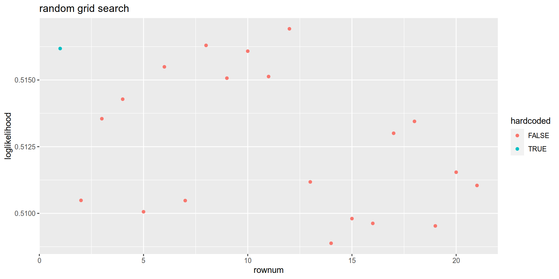
Example #2 Bayesian optimization using mlrMBO
This tutorial builds on the mlrMBO vignette
First, we need to define the objective function that the bayesian search will try to maximise. In this case we want to maximise the log likelihood of the out of fold predictions.
# objective function: we want to maximise the log likelihood by tuning most parameters
obj.fun  <- smoof::makeSingleObjectiveFunction(
  name = "xgb_cv_bayes",
  fn =   function(x){
    set.seed(12345)
    cv <- xgb.cv(params = list(
      booster          = "gbtree",
      eta              = x["eta"],
      max_depth        = x["max_depth"],
      min_child_weight = x["min_child_weight"],
      gamma            = x["gamma"],
      subsample        = x["subsample"],
      colsample_bytree = x["colsample_bytree"],
      objective        = 'count:poisson',
      eval_metric     = "poisson-nloglik"),
      data = mydb_xgbmatrix,
      nround = 30,
      folds=  cv_folds,
      monotone_constraints = myConstraint$sens,
      prediction = FALSE,
      showsd = TRUE,
      early_stopping_rounds = 10,
      verbose = 0)

    cv$evaluation_log[, max(test_poisson_nloglik_mean)]
  },
  par.set = makeParamSet(
    makeNumericParam("eta",              lower = 0.001, upper = 0.05),
    makeNumericParam("gamma",            lower = 0,     upper = 5),
    makeIntegerParam("max_depth",        lower= 1,      upper = 10),
    makeIntegerParam("min_child_weight", lower= 1,      upper = 10),
    makeNumericParam("subsample",        lower = 0.2,   upper = 1),
    makeNumericParam("colsample_bytree", lower = 0.2,   upper = 1)
  ),
  minimize = FALSE
)
After this, we generate the design, which are a set of hyperparameters that will be tested before starting the bayesian optimization. Here we generate only 10 sets, but mlrMBOwould normally generate 4 times the number of parameters. I also force my simon_params to be part of the design because I want to make sure at least one of of sets generated is good.
# generate an optimal design with only 10  points
des = generateDesign(n=10,
                     par.set = getParamSet(obj.fun),
                     fun = lhs::randomLHS)  ## . If no design is given by the user, mlrMBO will generate a maximin Latin Hypercube Design of size 4 times the number of the black-box function’s parameters.
# i still want my favorite hyperparameters to be tested
simon_params <- data.frame(max_depth = 6,
                           colsample_bytree= 0.8,
                           subsample = 0.8,
                           min_child_weight = 3,
                           eta  = 0.01,
                           gamma = 0) %>% as_tibble()
#final design  is a combination of latin hypercube optimization and my own preferred set of parameters
final_design =  simon_params  %>% bind_rows(des)
# bayes will have 10 additional iterations
control = makeMBOControl()
control = setMBOControlTermination(control, iters = 10)
Run the bayesian search:
if ( switch_generate_interim_data){
  run = mbo(fun = obj.fun,
            design = final_design,
            control = control,
            show.info = TRUE)
  write_rds( run, here::here("content/post/data/interim/run.rds"))
} else {
  run <- read_rds(here::here("content/post/data/interim/run.rds"))
}
# print a summary with run
#run
# return best model hyperparameters using run$x
# return best log likelihood using run$y
# return all results using run$opt.path$env$path
run$opt.path$env$path %>%
mutate(Round = row_number()) %>%
mutate(type = case_when(
Round==1 ~ "1- hardcoded",
Round<= 11 ~ "2 -design ",
TRUE ~ "3 - mlrMBO optimization")) %>%
ggplot(aes(x= Round, y= y, color= type)) +
geom_point() +
labs(title = "mlrMBO optimization")+
ylab("loglikelihood")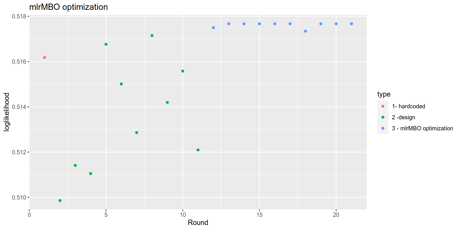
Conclusion:
Bayesian optimization does generate better models, but it might be overkill if you aren’t participating in a kaggle. The table below shows the log likelihood of the best model found using the random grid and the mlrMBO and compares it my simon params.
| type | loglikelihood | max_depth | colsample_bytree | subsample | min_child_weight | eta | gamma |
|---|---|---|---|---|---|---|---|
| simon params | 0.5161797 | 6 | 0.8000000 | 0.8000000 | 3 | 0.0100000 | 0.000000 |
| random_grid | 0.5169187 | 3 | 0.6796527 | 0.8889676 | 9 | 0.0055361 | 3.531973 |
| mlrMBO | 0.5176710 | 2 | 0.2768691 | 0.6206134 | 2 | 0.0010027 | 1.875530 |
Code
The code that generated this document is located at
https://github.com/SimonCoulombe/snippets/blob/master/content/post/2019-1-09-bayesian.Rmd
mlrMBO further reading
Here are some resources I used to build this post:
- Xgboost using MLR package
- Vignette: https://mlrmbo.mlr-org.com/articles/supplementary/machine_learning_with_mlrmbo.html , how to use lrMBO with mlr. I dont think you can do poisson regression using mlr.
- Parameter tuning with mlrHyperopt
- Train R ML models efficiently with mlr
Appendix: (NOT RECOMMENDED) Bayesian optimization using rBayesianOptimization
Here I show how to do an equivalent optimization using rBaysianOptimization. I do not recommend using this package because it recycles hyperparameters and hasnt been updated on github since 2016.
First, we have to define a special function that return a list of two values that will be returned to the bayesian optimiser:
- “Score” should be the metrics to be maximized ,
- “Pred” should be the validation/cross-valiation prediction for ensembling / stacking. We can set it to 0 to save on memory.
This function will be named xgb_cv_bayes :
xgb_cv_bayes <-
  function(max_depth=4,
           min_child_weight=1,
           gamma=0,
           eta=0.01,
           subsample = 0.6,
           colsample_bytree =0.6,
           nrounds = 200,
           early_stopping_rounds = 50 ){
    set.seed(1234)
    cv <- xgb.cv(params = list(
      booster = "gbtree",
      eta = eta,
      max_depth = max_depth,
      min_child_weight = min_child_weight,
      gamma = gamma,
      subsample = subsample,
      colsample_bytree = colsample_bytree,
      objective = 'count:poisson',
      eval_metric = "poisson-nloglik"),
      data = mydb_xgbmatrix,
      nround = nrounds,
      folds=  cv_folds,
      monotone_constraints = myConstraint$sens,
      prediction = FALSE,
      showsd = TRUE,
      early_stopping_rounds = 50,
      verbose = 0)

    list(Score = cv$evaluation_log[, max(test_poisson_nloglik_mean)],
         Pred = 0)
  }
We then launch BayesianOptimization, specifying:
- the function to optimise (xgb_cv_bayes),
- the hyperparameters (bounds) ,
- the number of iterations, n_iter,
The optimization function needs some points for initialisation. We pass one of the two following parameters:
- init_points , start from scratch using this number of randomly generated hyperparameter sets, or
- init_grid_dt use the knowledge from a previous run.
rBayesianOptimization from scratch
Here is an example “from scratch”.
if ( switch_generate_interim_data){
  bayesian_results <- rBayesianOptimization::BayesianOptimization(
    FUN = xgb_cv_bayes,
    bounds = list(max_depth = c(2L, 10L),
                  colsample_bytree = c(0.3, 1),
                  subsample = c(0.3,1),
                  min_child_weight = c(1L, 10L),
                  eta = c(0.001, 0.03),
                  gamma = c(0, 5)),
    init_grid_dt = NULL, init_points = 4,
    n_iter = 7,
    acq = "ucb", kappa = 2.576, eps = 0.0,
    verbose = TRUE)

  write_rds(bayesian_results, here::here("content/post/data/interim/bayesian_results.rds"))
} else {bayesian_results <- read_rds( here::here("content/post/data/interim/bayesian_results.rds"))}knitr::kable(bayesian_results$History)| Round | max_depth | colsample_bytree | subsample | min_child_weight | eta | gamma | Value |
|---|---|---|---|---|---|---|---|
| 1 | 10 | 0.3968879 | 0.5821038 | 1 | 0.0103839 | 2.0822446 | 0.5161180 |
| 2 | 3 | 0.8768590 | 0.7366128 | 9 | 0.0135183 | 4.8732243 | 0.5155987 |
| 3 | 3 | 0.7481389 | 0.5984350 | 8 | 0.0034476 | 0.2085726 | 0.5172650 |
| 4 | 7 | 0.6551866 | 0.9697193 | 5 | 0.0045494 | 1.1913145 | 0.5170820 |
| 5 | 4 | 0.9726352 | 0.7399260 | 4 | 0.0010000 | 1.4119299 | 0.5176710 |
| 6 | 4 | 0.9726295 | 0.7399255 | 4 | 0.0010000 | 1.4119589 | 0.5176710 |
| 7 | 4 | 0.9726215 | 0.7399260 | 4 | 0.0010000 | 1.4119589 | 0.5176710 |
| 8 | 4 | 0.9726190 | 0.7399260 | 4 | 0.0010000 | 1.4119589 | 0.5176710 |
| 9 | 4 | 0.9726177 | 0.7399260 | 4 | 0.0010000 | 1.4119589 | 0.5176710 |
| 10 | 4 | 0.9726167 | 0.7399260 | 4 | 0.0010000 | 1.4119589 | 0.5176710 |
| 11 | 5 | 0.3701890 | 0.8769125 | 8 | 0.0299810 | 3.9359835 | 0.5128937 |
bayesian_results$History  %>%
  mutate(type = case_when(
    Round<= 4  ~ "1- init_points",
    Round<= 11 ~ "2 -n_iter",
    TRUE ~ "wtf")) %>%
  ggplot(aes(x= Round, y= Value, color= type)) + geom_point()+
  labs(title = "bayesian from scratch")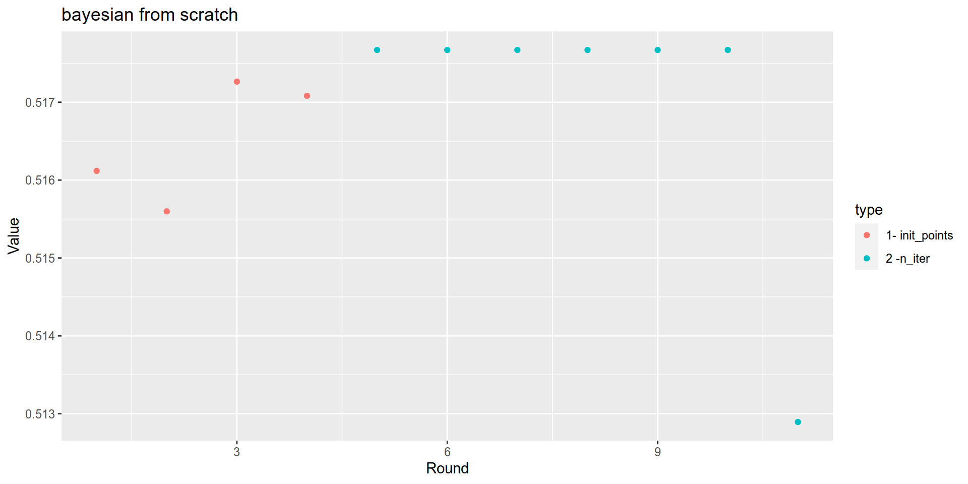
rBayesianOptimization resuming from previous runs
init_grid_dt is a data frame with the same columns as bounds plus a Valuecolumn which correspond to the log likelihood we calculated earlier.
… resuming from random grid
Here is an example resuming from the random grid of example #1
init_grid <- random_grid_results$data %>%
  bind_rows() %>%
  add_column(Value = random_grid_results$Score)   %>%
  select(max_depth, colsample_bytree, subsample, min_child_weight, eta, gamma, Value)
knitr::kable(init_grid)| max_depth | colsample_bytree | subsample | min_child_weight | eta | gamma | Value |
|---|---|---|---|---|---|---|
| 6 | 0.8000000 | 0.8000000 | 3 | 0.0100000 | 0.000000 | 0.5161797 |
| 4 | 0.3697140 | 0.7176482 | 3 | 0.0447509 | 0.000000 | 0.5104867 |
| 5 | 0.7213390 | 0.8263462 | 5 | 0.0259997 | 0.000000 | 0.5135480 |
| 7 | 0.3004441 | 0.6424290 | 4 | 0.0215211 | 0.000000 | 0.5142803 |
| 4 | 0.4137765 | 0.6237757 | 7 | 0.0474252 | 0.000000 | 0.5100597 |
| 7 | 0.5088913 | 0.8314850 | 3 | 0.0141615 | 0.000000 | 0.5154927 |
| 7 | 0.2107123 | 0.2186650 | 5 | 0.0446673 | 0.000000 | 0.5104790 |
| 6 | 0.5059104 | 0.5817841 | 8 | 0.0093015 | 0.000000 | 0.5162973 |
| 6 | 0.8957527 | 0.7858510 | 1 | 0.0167293 | 0.000000 | 0.5150687 |
| 3 | 0.4722792 | 0.7541852 | 9 | 0.0105983 | 0.000000 | 0.5160807 |
| 4 | 0.5856641 | 0.5820957 | 4 | 0.0163778 | 0.000000 | 0.5151290 |
| 3 | 0.6796527 | 0.8889676 | 9 | 0.0055361 | 3.531973 | 0.5169187 |
| 6 | 0.5948330 | 0.5504777 | 4 | 0.0405373 | 2.702602 | 0.5111790 |
| 4 | 0.3489741 | 0.3958378 | 4 | 0.0545762 | 9.926841 | 0.5088790 |
| 6 | 0.8618987 | 0.2565432 | 5 | 0.0487349 | 6.334933 | 0.5098037 |
| 5 | 0.7347734 | 0.2795729 | 9 | 0.0498385 | 2.132081 | 0.5096243 |
| 6 | 0.8353919 | 0.4530174 | 9 | 0.0293165 | 1.293724 | 0.5130033 |
| 7 | 0.2863549 | 0.6149074 | 4 | 0.0266050 | 4.781180 | 0.5134483 |
| 4 | 0.7789688 | 0.7296041 | 8 | 0.0506522 | 9.240745 | 0.5095290 |
| 6 | 0.5290195 | 0.5254641 | 10 | 0.0382960 | 5.987610 | 0.5115423 |
| 7 | 0.8567570 | 0.9303007 | 5 | 0.0412834 | 9.761707 | 0.5110460 |
if (switch_generate_interim_data){
  bayesian_results_continued_from_randomgrid <-
    BayesianOptimization(xgb_cv_bayes,
                         bounds = list(max_depth = c(2L, 10L),
                                       colsample_bytree = c(0.3, 1),
                                       subsample = c(0.3,1),
                                       min_child_weight = c(1L, 10L),
                                       eta = c(0.001, 0.03),
                                       gamma = c(0, 5)),
                         init_grid_dt = init_grid, init_points = 0,
                         n_iter = 5,
                         acq = "ucb", kappa = 2.576, eps = 0.0,
                         verbose = TRUE)

  write_rds(bayesian_results_continued_from_randomgrid,
            here::here("content/post/data/interim/bayesian_results_continued_from_randomgrid.rds"))
} else {

  bayesian_results_continued_from_randomgrid <- read_rds(
    here::here("content/post/data/interim/bayesian_results_continued_from_randomgrid.rds"))
}
… resuming from previous rBayesianOptimization
We can also resume from a brevious rBayesianOptimization run using the $History value it returns. In the example below, we will resume from the previous bayesian search that was itself build upon the random grid search.
init_grid <- bayesian_results_continued_from_randomgrid$History %>% select(-Round)
knitr::kable(init_grid)| max_depth | colsample_bytree | subsample | min_child_weight | eta | gamma | Value |
|---|---|---|---|---|---|---|
| 6 | 0.8000000 | 0.8000000 | 3 | 0.0100000 | 0.0000000 | 0.5161797 |
| 4 | 0.3697140 | 0.7176482 | 3 | 0.0447509 | 0.0000000 | 0.5104867 |
| 5 | 0.7213390 | 0.8263462 | 5 | 0.0259997 | 0.0000000 | 0.5135480 |
| 7 | 0.3004441 | 0.6424290 | 4 | 0.0215211 | 0.0000000 | 0.5142803 |
| 4 | 0.4137765 | 0.6237757 | 7 | 0.0474252 | 0.0000000 | 0.5100597 |
| 7 | 0.5088913 | 0.8314850 | 3 | 0.0141615 | 0.0000000 | 0.5154927 |
| 7 | 0.2107123 | 0.2186650 | 5 | 0.0446673 | 0.0000000 | 0.5104790 |
| 6 | 0.5059104 | 0.5817841 | 8 | 0.0093015 | 0.0000000 | 0.5162973 |
| 6 | 0.8957527 | 0.7858510 | 1 | 0.0167293 | 0.0000000 | 0.5150687 |
| 3 | 0.4722792 | 0.7541852 | 9 | 0.0105983 | 0.0000000 | 0.5160807 |
| 4 | 0.5856641 | 0.5820957 | 4 | 0.0163778 | 0.0000000 | 0.5151290 |
| 3 | 0.6796527 | 0.8889676 | 9 | 0.0055361 | 3.5319727 | 0.5169187 |
| 6 | 0.5948330 | 0.5504777 | 4 | 0.0405373 | 2.7026015 | 0.5111790 |
| 4 | 0.3489741 | 0.3958378 | 4 | 0.0545762 | 9.9268406 | 0.5088790 |
| 6 | 0.8618987 | 0.2565432 | 5 | 0.0487349 | 6.3349326 | 0.5098040 |
| 5 | 0.7347734 | 0.2795729 | 9 | 0.0498385 | 2.1320814 | 0.5096243 |
| 6 | 0.8353919 | 0.4530174 | 9 | 0.0293165 | 1.2937235 | 0.5130033 |
| 7 | 0.2863549 | 0.6149074 | 4 | 0.0266050 | 4.7811803 | 0.5134483 |
| 4 | 0.7789688 | 0.7296041 | 8 | 0.0506522 | 9.2407447 | 0.5095290 |
| 6 | 0.5290195 | 0.5254641 | 10 | 0.0382960 | 5.9876097 | 0.5115423 |
| 7 | 0.8567570 | 0.9303007 | 5 | 0.0412834 | 9.7617069 | 0.5110460 |
| 6 | 0.8558321 | 0.8749248 | 5 | 0.0071978 | 4.4704073 | 0.5166430 |
| 9 | 0.4646962 | 0.5923405 | 7 | 0.0053862 | 0.2069889 | 0.5169443 |
| 6 | 0.3418069 | 0.8590210 | 2 | 0.0035004 | 2.8826489 | 0.5172560 |
| 10 | 0.4647044 | 0.6429887 | 7 | 0.0049578 | 5.0000000 | 0.5170143 |
| 2 | 0.7317249 | 0.5751665 | 8 | 0.0010000 | 4.7603658 | 0.5176710 |
if (switch_generate_interim_data){
  bayesian_results_continued_from_bayesian <-
    BayesianOptimization(xgb_cv_bayes,
                         bounds = list(max_depth = c(2L, 10L),
                                       colsample_bytree = c(0.3, 1),
                                       subsample = c(0.3,1),
                                       min_child_weight = c(1L, 10L),
                                       eta = c(0.001, 0.03),
                                       gamma = c(0, 5)),
                         init_grid_dt =init_grid , init_points = 0,
                         n_iter = 5,
                         acq = "ucb", kappa = 2.576, eps = 0.0,
                         verbose = TRUE)
  write_rds(bayesian_results_continued_from_bayesian,here::here("content/post/data/interim/bayesian_results_continued_from_bayesian.rds"))
} else {
  bayesian_results_continued_from_bayesian <- read_rds(
    here::here("content/post/data/interim/bayesian_results_continued_from_bayesian.rds"))
}
bayesian_results_continued_from_bayesian$History %>%
mutate(type = case_when(
Round==1 ~ "1- hardcoded",
Round<= 21 ~ "2 -random grid ",
Round <= 26 ~ "3 - rbayesianoptimization run #1 resuming from random grid",
TRUE ~ "4 - rbayesianoptimization run #2 resuming from bayesian run 1")) %>%
ggplot(aes(x= Round, y= Value, color= type)) +
geom_point()+
labs(title = "rBayesianOptimization")+
ylab("loglikelihood")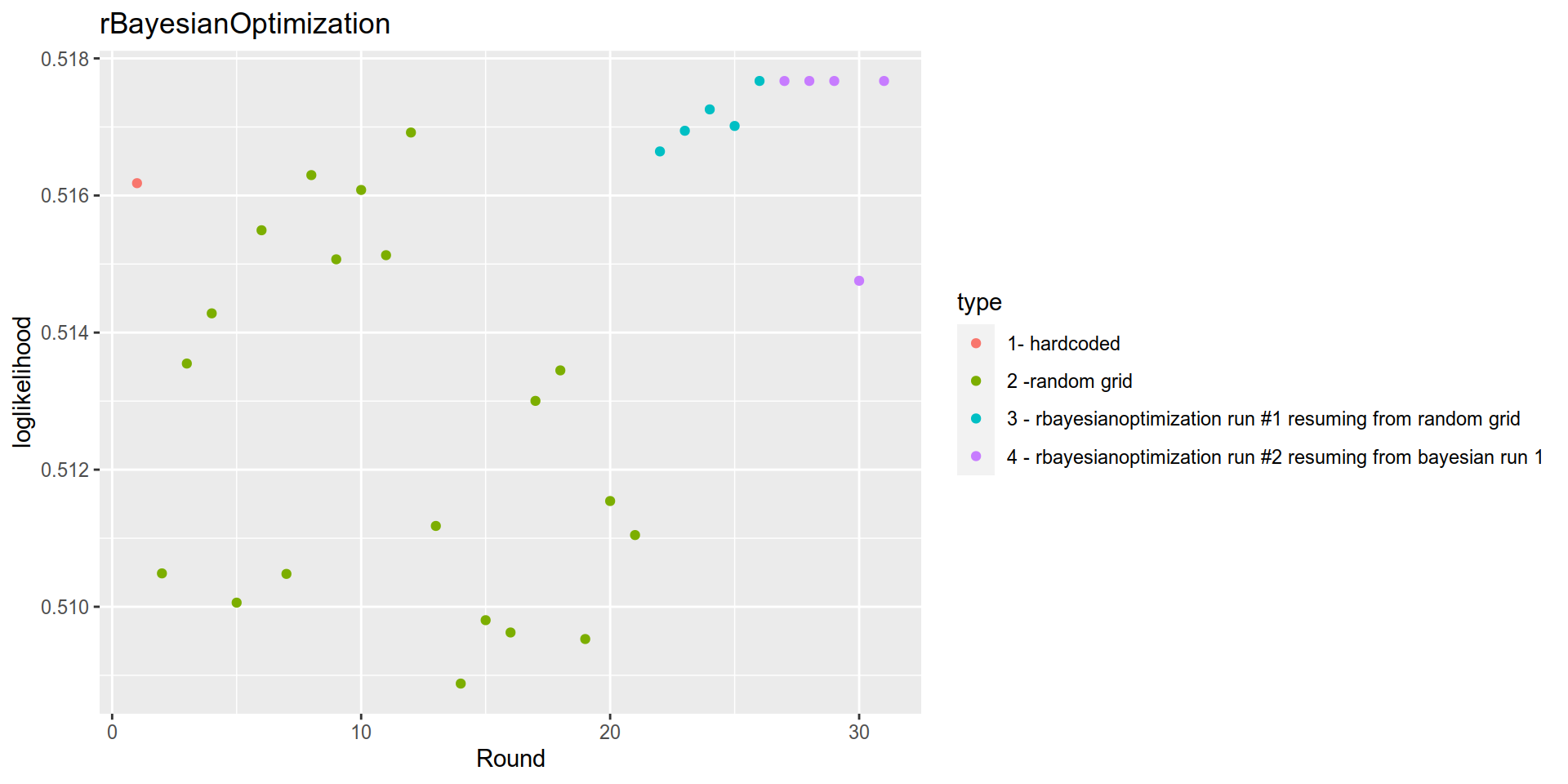
Conclusion
The table below shows the loglikelihood and hyperparameters for the hardcoded simon_param model, and the best models found by random search, mlrMBO and rBayesianOptimisation.
Bayesian optimization using mlrMBO and rBayesianOptimization both yield the best results. The gain in loglikelihood above the “hardcoded” simon_param or the random search isnt that great, however, so it may not be necessary to implement mlrMBO in a non-kaggle setting.
hardcoded <- random_grid_results[1,] %>%
  pull(data) %>% .[[1]] %>%
  mutate(type = "hardcoded") %>%
  mutate(loglikelihood= random_grid_results[1,"Score"] %>% as.numeric())
best_random <- random_grid_results %>%
  filter(Score == max(Score)) %>% pull(data) %>% .[[1]] %>%
  mutate(type = "random_grid") %>%
  mutate(loglikelihood = max(random_grid_results$Score))

best_mlrMBO <- run$opt.path$env$path  %>%
  filter(y == max(y))  %>%
  mutate(type = "mlrMBO") %>%
  mutate(loglikelihood= run$y ) %>%
  head(1)
best_rBayesianOptimization <-
  bayesian_results_continued_from_bayesian$History %>%
  filter(Value == max(Value)) %>%
  mutate(type = "rBayesianOptimization") %>%
  mutate(loglikelihood = max(bayesian_results_continued_from_bayesian$History$Value))
hardcoded %>%
  bind_rows(best_random) %>%
  bind_rows(best_mlrMBO) %>%
  bind_rows(best_rBayesianOptimization) %>%
select(type,loglikelihood, max_depth, colsample_bytree, subsample,min_child_weight,eta, gamma) %>% knitr::kable()| type | loglikelihood | max_depth | colsample_bytree | subsample | min_child_weight | eta | gamma |
|---|---|---|---|---|---|---|---|
| hardcoded | 0.5161797 | 6 | 0.8000000 | 0.8000000 | 3 | 0.0100000 | 0.000000 |
| random_grid | 0.5169187 | 3 | 0.6796527 | 0.8889676 | 9 | 0.0055361 | 3.531973 |
| mlrMBO | 0.5176710 | 2 | 0.2768691 | 0.6206134 | 2 | 0.0010027 | 1.875530 |
| rBayesianOptimization | 0.5176710 | 2 | 0.7317249 | 0.5751665 | 8 | 0.0010000 | 4.760366 |
| rBayesianOptimization | 0.5176710 | 10 | 1.0000000 | 0.3000000 | 1 | 0.0010000 | 3.249263 |