NHL: And the most useful player of the league is...
Hey everyone,
We all know that the good old plus/minus is flawed. Most notably, it doesn’t take into account the quality of your teammates or that of the opposition. So here is my idea: why not use a Poisson regression?
The Poisson regression is a special type of regression where the response variable is a count. For example, ecologists will model the number of fish in samples of a lake of varying volume, accounting for different characteristics of that volume, and actuaries will model the number of claims someone will make during a car insurance policy of varying duration accounting for different characteristics of the driver.
My plan is to find out which factors (players) influence the rate at which a team will score during a shift taking into account the 6 players (including goalie) on that team, and the 6 players against them.
More precisely, I model goals on 1003 “offense player dummies” and 1003 “defense player dummies” and I use duration of the shift as an offset variable. This will return an “offense strength” and a “defense strength” for each of the 1003 players that players during the 2018-2019 season.
As usual, the code is available on github.
If your team doesnt make it to the end of the playoffs, make sure to use my pub crawling app to get you drunk and home optimally.
Disclaimer: I haven’t watched a game with passion since Kovalev faked an injury against my beloved Nordiques in the year we were meant to win the damn cup. I also haven’t followed hockey advanced analytics ever, so this may be a very old or very bad idea, but I still thought I’d share it because I had fun building this :).
The model
Let’s look at this shift chart from a Montreal vs Toronto game.
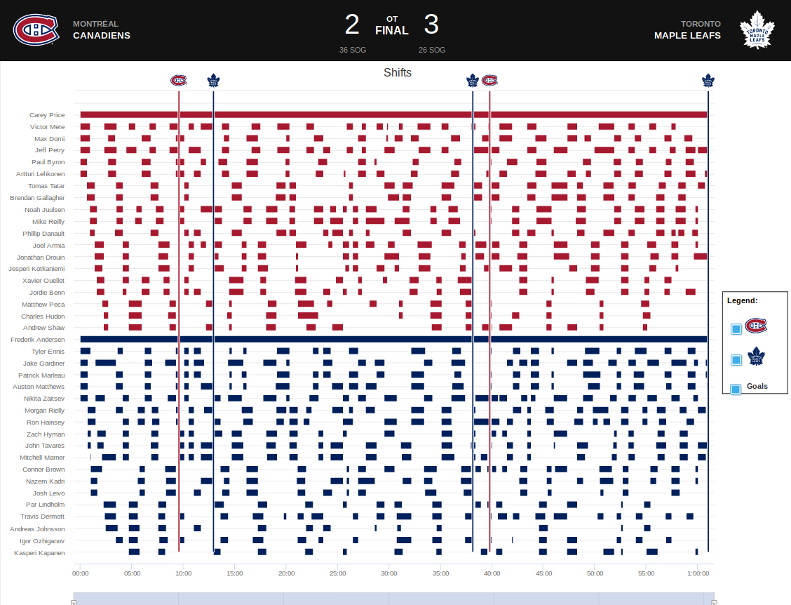 I define a “shift” as a period of time where all the players of both team are identical.
The first shift is Price-Mete-Domi-Petry-Byron-Lehkonen vs Andersen-Ennis,Gardiner-Marleau-Matthews-Zaitsev and it lasts 38 seconds, until Byron and Lehkonen leave the ice.
The second shift is Price-Mete-Domi-Petry-Tatar-Gallagher vs Andersen-Ennis,Gardiner-Marleau-Matthews-Zaitsev and it only lasts 4 seconds, until the Leafs replace 4 players at 00:42.
The third shift is Price-Mete-Domi-Petry-Tatar-Gallagher vs Andersen-Ennis-Rielly-Hainsey-Hyman-Tavares and it lasts 14s, until the Mete-Domi-Petry line is replaced at 00:56.
Etc..
During a shift, both teams have a chance to score a goal, so I the model includes two lines for each shift, one for each team attempting to score. The columns included in the model are “did the team score?”, “how long did the shift last in seconds?” and “who was playing on offense and defense” ?
In the case of our first shift, the two lines created would be as follow:
0 goal, 38 seconds, offense: Price-Mete-Domi-Petry-Byron-Lehkonen , defense: Andersen-Ennis,Gardiner-Marleau-Matthews-Zaitsev.
0 goal, 38 seconds, offense: Andersen-Ennis,Gardiner-Marleau-Matthews-Zaitsev , defense: Price-Mete-Domi-Petry-Byron-Lehkonen.
For the model, I only keep “shifts” where the strength is an even 5 on 5 (plus goalies).
There are many ways to model a Poisson regression. My go-to solution would have been to use a Generalized Linear Model (GLM) because it would have output a coefficient for each player for defense and offense and would have made the players directly comparable. However, I quickly ran into issues because the GLM had a hard time digesting the 2006 features and 622 502 rows and wouldn’t converge. The alternative was to use a more powerful but less straightforward Gradien-Boosting model (GBM). I chose to use LightGBM because its fast and has a low memory need, which made it possible to run on my 32GB RAM computer.
To get the offensive contribution of the player accounting for teammates and opposition, I use the model to predict how many goals per hour an average team including this player would score against an average team. Inversely, to get the defensive contribution of the player accounting for teammates and opposition, I use the model to predict how many goals per hour an average team would score against an average team including this player.
More precisely, I score the model using a value of “0” for all features, except for the variable I am interested in (ex: against_player_PK_Subban), which is set to “1”.
Getting the data
I create a few functions to allow me to download the data from NHL.com’s API. They are on the github repo mentionned above and have straightforward names such as get_schedule(), get_player_data(), get_data() and get_shift_data().
The results !!
The average team will score an average of 2.58 goals per 60 minutes when playing at 5 on 5 against an average team.
Swap John Carlson and your team will suddenly score at a rate of average of 3.76 goals per 60 minutes played and suffer a slightly increased goal rate of 2.69.
Crosby (3.55) and Kucherov (3.48) are slightly behind. They were kind of obvious, but what is Carlson doing there? He is a defenseman! Maybe whoever is in front of him will receive better passes and play offense with more confidence, allowing them to score goals.
| rank | player | position | team | offense | defense | differential | hours_played |
|---|---|---|---|---|---|---|---|
| 1 | John Carlson | D | Washington Capitals | 3.76 | 2.69 | 1.07 | 37.10 |
| 2 | Sidney Crosby | C | Pittsburgh Penguins | 3.55 | 2.58 | 0.97 | 29.73 |
| 3 | Nikita Kucherov | R | Tampa Bay Lightning | 3.48 | 2.58 | 0.89 | 28.89 |
| 4 | Patrick Kane | R | Chicago Blackhawks | 3.44 | 2.60 | 0.84 | 30.89 |
| 5 | Leon Draisaitl | C | Edmonton Oilers | 3.38 | 2.97 | 0.41 | 31.46 |
| 6 | Morgan Rielly | D | Toronto Maple Leafs | 3.23 | 2.58 | 0.65 | 35.25 |
| 7 | Mark Stone | R | Vegas Golden Knights | 3.23 | 2.58 | 0.64 | 28.58 |
| 8 | John Tavares | C | Toronto Maple Leafs | 3.22 | 2.71 | 0.51 | 28.98 |
| 9 | Patrice Bergeron | C | Boston Bruins | 3.21 | 2.58 | 0.63 | 27.14 |
| 10 | Tomas Hertl | C | San Jose Sharks | 3.21 | 2.74 | 0.47 | 31.99 |
| 11 | Matt Duchene | C | Columbus Blue Jackets | 3.21 | 2.68 | 0.53 | 26.22 |
| 12 | Chris Kreider | L | New York Rangers | 3.13 | 2.58 | 0.55 | 23.41 |
| 13 | Artemi Panarin | L | Columbus Blue Jackets | 3.10 | 2.58 | 0.51 | 30.34 |
| 14 | Connor McDavid | C | Edmonton Oilers | 3.09 | 2.81 | 0.28 | 30.24 |
| 15 | Alexander Radulov | R | Dallas Stars | 3.09 | 2.58 | 0.51 | 27.88 |
| 16 | Claude Giroux | C | Philadelphia Flyers | 3.08 | 2.58 | 0.49 | 29.92 |
| 17 | Andrew Shaw | R | Montréal Canadiens | 3.06 | 2.58 | 0.48 | 17.06 |
| 18 | Jeff Skinner | L | Buffalo Sabres | 3.04 | 2.58 | 0.45 | 25.79 |
| 19 | Sebastian Aho | C | Carolina Hurricanes | 3.03 | 2.58 | 0.45 | 33.45 |
| 20 | Ryan Murray | D | Columbus Blue Jackets | 3.01 | 2.58 | 0.42 | 20.43 |
| 21 | Evgenii Dadonov | R | Florida Panthers | 3.00 | 2.58 | 0.41 | 25.62 |
| 22 | Alex DeBrincat | L | Chicago Blackhawks | 2.99 | 2.71 | 0.28 | 24.65 |
| 23 | Max Domi | C | Montréal Canadiens | 2.99 | 2.58 | 0.41 | 24.24 |
| 24 | Phillip Danault | C | Montréal Canadiens | 2.97 | 2.58 | 0.38 | 24.54 |
| 25 | Taylor Hall | L | New Jersey Devils | 2.96 | 2.62 | 0.34 | 11.03 |
| 26 | Aleksander Barkov | C | Florida Panthers | 2.95 | 2.63 | 0.32 | 31.17 |
| 27 | Alex Ovechkin | L | Washington Capitals | 2.95 | 2.91 | 0.05 | 31.30 |
| 28 | Ryan Johansen | C | Nashville Predators | 2.95 | 2.77 | 0.18 | 28.76 |
| 29 | Tony DeAngelo | D | New York Rangers | 2.92 | 2.58 | 0.33 | 20.06 |
| 30 | Sean Couturier | C | Philadelphia Flyers | 2.92 | 2.85 | 0.07 | 30.10 |
The players that have the best defensive impact (reducing the rate at which the opponent score) are Andrew Cogliano (DAL), Derek Ryan (CGY)and Danton Heinen (BOS). I honestly don’t know them, so let me know what you think.
| rank | player | position | team | offense | defense | differential | hours_played |
|---|---|---|---|---|---|---|---|
| 1 | Andrew Cogliano | C | Dallas Stars | 2.44 | 1.92 | 0.51 | 19.98 |
| 2 | Derek Ryan | C | Calgary Flames | 2.58 | 1.93 | 0.65 | 20.29 |
| 3 | Danton Heinen | C | Boston Bruins | 2.58 | 1.97 | 0.61 | 23.14 |
| 4 | Sean Kuraly | C | Boston Bruins | 2.58 | 2.00 | 0.58 | 21.18 |
| 5 | Brandon Carlo | D | Boston Bruins | 2.58 | 2.02 | 0.56 | 33.50 |
| 6 | Tobias Rieder | R | Edmonton Oilers | 1.37 | 2.04 | -0.67 | 14.46 |
| 7 | Cal Petersen | G | Los Angeles Kings | 2.58 | 2.08 | 0.50 | 10.37 |
| 8 | Jordan Binnington | G | St. Louis Blues | 2.58 | 2.09 | 0.49 | 54.02 |
| 9 | Adam Pelech | D | New York Islanders | 2.58 | 2.15 | 0.43 | 27.55 |
| 10 | Jason Demers | D | Arizona Coyotes | 2.58 | 2.18 | 0.41 | 11.92 |
| 11 | Colton Parayko | D | St. Louis Blues | 2.58 | 2.18 | 0.40 | 40.79 |
| 12 | Andrew Copp | C | Winnipeg Jets | 2.69 | 2.19 | 0.50 | 15.74 |
| 13 | Sven Andrighetto | R | Colorado Avalanche | 2.58 | 2.24 | 0.35 | 12.74 |
| 14 | Petr Mrazek | G | Carolina Hurricanes | 2.58 | 2.27 | 0.31 | 50.84 |
| 15 | Connor Brown | R | Toronto Maple Leafs | 2.58 | 2.28 | 0.30 | 20.86 |
| 16 | Carey Price | G | Montréal Canadiens | 2.58 | 2.29 | 0.29 | 64.74 |
| 17 | Matt Martin | L | New York Islanders | 2.30 | 2.29 | 0.00 | 14.67 |
| 18 | Nick Bonino | C | Nashville Predators | 2.58 | 2.32 | 0.26 | 24.12 |
| 19 | Conor Garland | R | Arizona Coyotes | 2.58 | 2.33 | 0.25 | 10.24 |
| 20 | Teuvo Teravainen | L | Carolina Hurricanes | 2.70 | 2.34 | 0.36 | 30.11 |
| 21 | Fredrik Claesson | D | New York Rangers | 2.58 | 2.35 | 0.24 | 10.87 |
| 22 | Esa Lindell | D | Dallas Stars | 2.58 | 2.35 | 0.23 | 39.84 |
| 23 | Oscar Fantenberg | D | Calgary Flames | 2.50 | 2.36 | 0.14 | 17.29 |
| 24 | Roman Polak | D | Dallas Stars | 2.58 | 2.36 | 0.22 | 29.44 |
| 25 | Brandon Tanev | L | Winnipeg Jets | 2.58 | 2.36 | 0.22 | 20.46 |
| 26 | Frederik Andersen | G | Toronto Maple Leafs | 2.58 | 2.38 | 0.21 | 65.47 |
| 27 | Scott Mayfield | D | New York Islanders | 2.58 | 2.38 | 0.20 | 27.70 |
| 28 | Marcus Pettersson | D | Pittsburgh Penguins | 2.58 | 2.38 | 0.20 | 25.13 |
| 29 | Brett Pesce | D | Carolina Hurricanes | 2.58 | 2.39 | 0.19 | 31.33 |
| 30 | Jack Campbell | G | Los Angeles Kings | 2.58 | 2.40 | 0.18 | 26.24 |
Finally, who are the best of the best? Those who help their team score and prevent the other team from scoring? The difference between the offense and defense score is the expected amount of goals by which an average team employing that player for 60 minutes per game would win against an average team.
The best players are still Carlson, Crosby and Kucherov.
| rank | player | position | team | offense | defense | differential | hours_played |
|---|---|---|---|---|---|---|---|
| 1 | John Carlson | D | Washington Capitals | 3.76 | 2.69 | 1.07 | 37.10 |
| 2 | Sidney Crosby | C | Pittsburgh Penguins | 3.55 | 2.58 | 0.97 | 29.73 |
| 3 | Nikita Kucherov | R | Tampa Bay Lightning | 3.48 | 2.58 | 0.89 | 28.89 |
| 4 | Patrick Kane | R | Chicago Blackhawks | 3.44 | 2.60 | 0.84 | 30.89 |
| 5 | Derek Ryan | C | Calgary Flames | 2.58 | 1.93 | 0.65 | 20.29 |
| 6 | Morgan Rielly | D | Toronto Maple Leafs | 3.23 | 2.58 | 0.65 | 35.25 |
| 7 | Mark Stone | R | Vegas Golden Knights | 3.23 | 2.58 | 0.64 | 28.58 |
| 8 | Patrice Bergeron | C | Boston Bruins | 3.21 | 2.58 | 0.63 | 27.14 |
| 9 | Danton Heinen | C | Boston Bruins | 2.58 | 1.97 | 0.61 | 23.14 |
| 10 | Sean Kuraly | C | Boston Bruins | 2.58 | 2.00 | 0.58 | 21.18 |
| 11 | Brandon Carlo | D | Boston Bruins | 2.58 | 2.02 | 0.56 | 33.50 |
| 12 | Chris Kreider | L | New York Rangers | 3.13 | 2.58 | 0.55 | 23.41 |
| 13 | Matt Duchene | C | Columbus Blue Jackets | 3.21 | 2.68 | 0.53 | 26.22 |
| 14 | Artemi Panarin | L | Columbus Blue Jackets | 3.10 | 2.58 | 0.51 | 30.34 |
| 15 | Andrew Cogliano | C | Dallas Stars | 2.44 | 1.92 | 0.51 | 19.98 |
| 16 | John Tavares | C | Toronto Maple Leafs | 3.22 | 2.71 | 0.51 | 28.98 |
| 17 | Alexander Radulov | R | Dallas Stars | 3.09 | 2.58 | 0.51 | 27.88 |
| 18 | Cal Petersen | G | Los Angeles Kings | 2.58 | 2.08 | 0.50 | 10.37 |
| 19 | Andrew Copp | C | Winnipeg Jets | 2.69 | 2.19 | 0.50 | 15.74 |
| 20 | Claude Giroux | C | Philadelphia Flyers | 3.08 | 2.58 | 0.49 | 29.92 |
| 21 | Jordan Binnington | G | St. Louis Blues | 2.58 | 2.09 | 0.49 | 54.02 |
| 22 | Andrew Shaw | R | Montréal Canadiens | 3.06 | 2.58 | 0.48 | 17.06 |
| 23 | Tomas Hertl | C | San Jose Sharks | 3.21 | 2.74 | 0.47 | 31.99 |
| 24 | Jeff Skinner | L | Buffalo Sabres | 3.04 | 2.58 | 0.45 | 25.79 |
| 25 | Sebastian Aho | C | Carolina Hurricanes | 3.03 | 2.58 | 0.45 | 33.45 |
| 26 | Adam Pelech | D | New York Islanders | 2.58 | 2.15 | 0.43 | 27.55 |
| 27 | Ryan Murray | D | Columbus Blue Jackets | 3.01 | 2.58 | 0.42 | 20.43 |
| 28 | Evgenii Dadonov | R | Florida Panthers | 3.00 | 2.58 | 0.41 | 25.62 |
| 29 | Leon Draisaitl | C | Edmonton Oilers | 3.38 | 2.97 | 0.41 | 31.46 |
| 30 | Max Domi | C | Montréal Canadiens | 2.99 | 2.58 | 0.41 | 24.24 |
Here is the table for the goalies only. Controlling for the opposition and his defense, the best goaltender who played more than 10 hours appears to be Cal Petersen, who brings the average rate of goals against per 60 minutes down to a cool 2.08. What do you think?
| rank | player | position | team | offense | defense | differential | hours_played |
|---|---|---|---|---|---|---|---|
| 1 | Cal Petersen | G | Los Angeles Kings | 2.58 | 2.08 | 0.50 | 10.37 |
| 2 | Jordan Binnington | G | St. Louis Blues | 2.58 | 2.09 | 0.49 | 54.02 |
| 3 | Petr Mrazek | G | Carolina Hurricanes | 2.58 | 2.27 | 0.31 | 50.84 |
| 4 | Carey Price | G | Montréal Canadiens | 2.58 | 2.29 | 0.29 | 64.74 |
| 5 | Frederik Andersen | G | Toronto Maple Leafs | 2.58 | 2.38 | 0.21 | 65.47 |
| 6 | Jack Campbell | G | Los Angeles Kings | 2.58 | 2.40 | 0.18 | 26.24 |
| 7 | Marc-Andre Fleury | G | Vegas Golden Knights | 2.58 | 2.42 | 0.16 | 68.43 |
| 8 | Andrei Vasilevskiy | G | Tampa Bay Lightning | 2.58 | 2.43 | 0.16 | 57.38 |
| 9 | Ben Bishop | G | Dallas Stars | 2.58 | 2.47 | 0.11 | 57.53 |
| 10 | Robin Lehner | G | New York Islanders | 2.58 | 2.49 | 0.09 | 51.14 |
| 11 | Juuse Saros | G | Nashville Predators | 2.66 | 2.58 | 0.08 | 29.06 |
| 12 | Tuukka Rask | G | Boston Bruins | 2.58 | 2.51 | 0.07 | 65.38 |
| 13 | Thomas Greiss | G | New York Islanders | 2.58 | 2.52 | 0.06 | 38.88 |
| 14 | Pekka Rinne | G | Nashville Predators | 2.58 | 2.53 | 0.05 | 59.22 |
| 15 | Laurent Brossoit | G | Winnipeg Jets | 2.58 | 2.54 | 0.04 | 19.44 |
| 16 | Sergei Bobrovsky | G | Columbus Blue Jackets | 2.58 | 2.57 | 0.01 | 69.73 |
| 17 | Roberto Luongo | G | Florida Panthers | 2.58 | 2.58 | 0.00 | 39.15 |
| 18 | Craig Anderson | G | Ottawa Senators | 2.58 | 2.58 | 0.00 | 46.47 |
| 19 | Ryan Miller | G | Anaheim Ducks | 2.58 | 2.58 | 0.00 | 18.50 |
| 20 | Mike Smith | G | Calgary Flames | 2.58 | 2.58 | 0.00 | 45.36 |
| 21 | Curtis McElhinney | G | Carolina Hurricanes | 2.58 | 2.58 | 0.00 | 37.47 |
| 22 | Cam Ward | G | Chicago Blackhawks | 2.58 | 2.58 | 0.00 | 31.41 |
| 23 | Corey Crawford | G | Chicago Blackhawks | 2.58 | 2.58 | 0.00 | 36.92 |
| 24 | Jimmy Howard | G | Detroit Red Wings | 2.58 | 2.58 | 0.00 | 50.94 |
| 25 | Jaroslav Halak | G | Boston Bruins | 2.58 | 2.58 | 0.00 | 38.51 |
| 26 | Brian Elliott | G | Philadelphia Flyers | 2.58 | 2.58 | 0.00 | 22.97 |
| 27 | Devan Dubnyk | G | Minnesota Wild | 2.58 | 2.58 | 0.00 | 64.33 |
| 28 | Cory Schneider | G | New Jersey Devils | 2.58 | 2.58 | 0.00 | 22.55 |
| 29 | Anton Khudobin | G | Dallas Stars | 2.58 | 2.58 | 0.00 | 37.22 |
| 30 | Jonathan Quick | G | Los Angeles Kings | 2.58 | 2.58 | 0.00 | 44.09 |
Caveats and conclusion
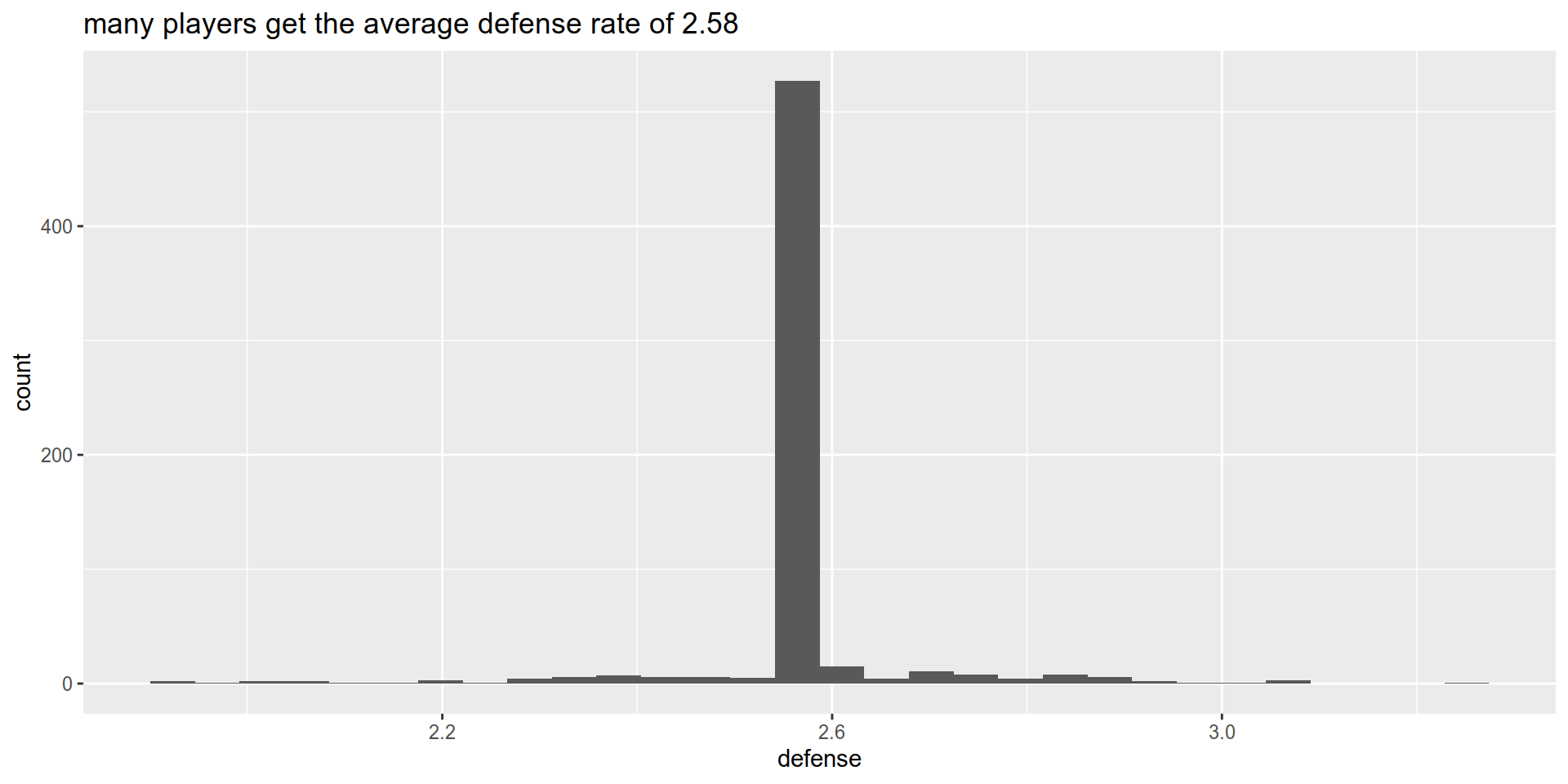
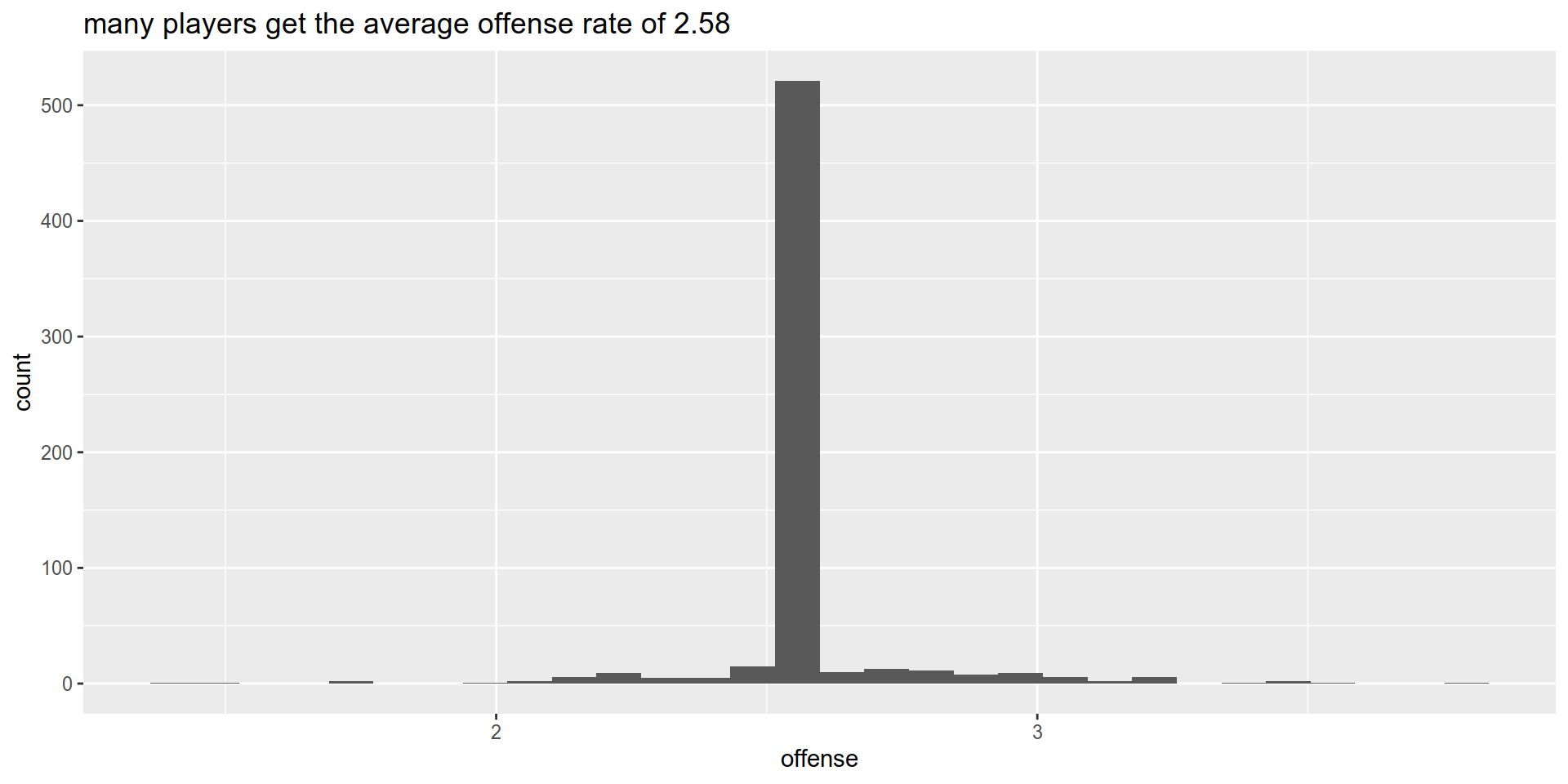
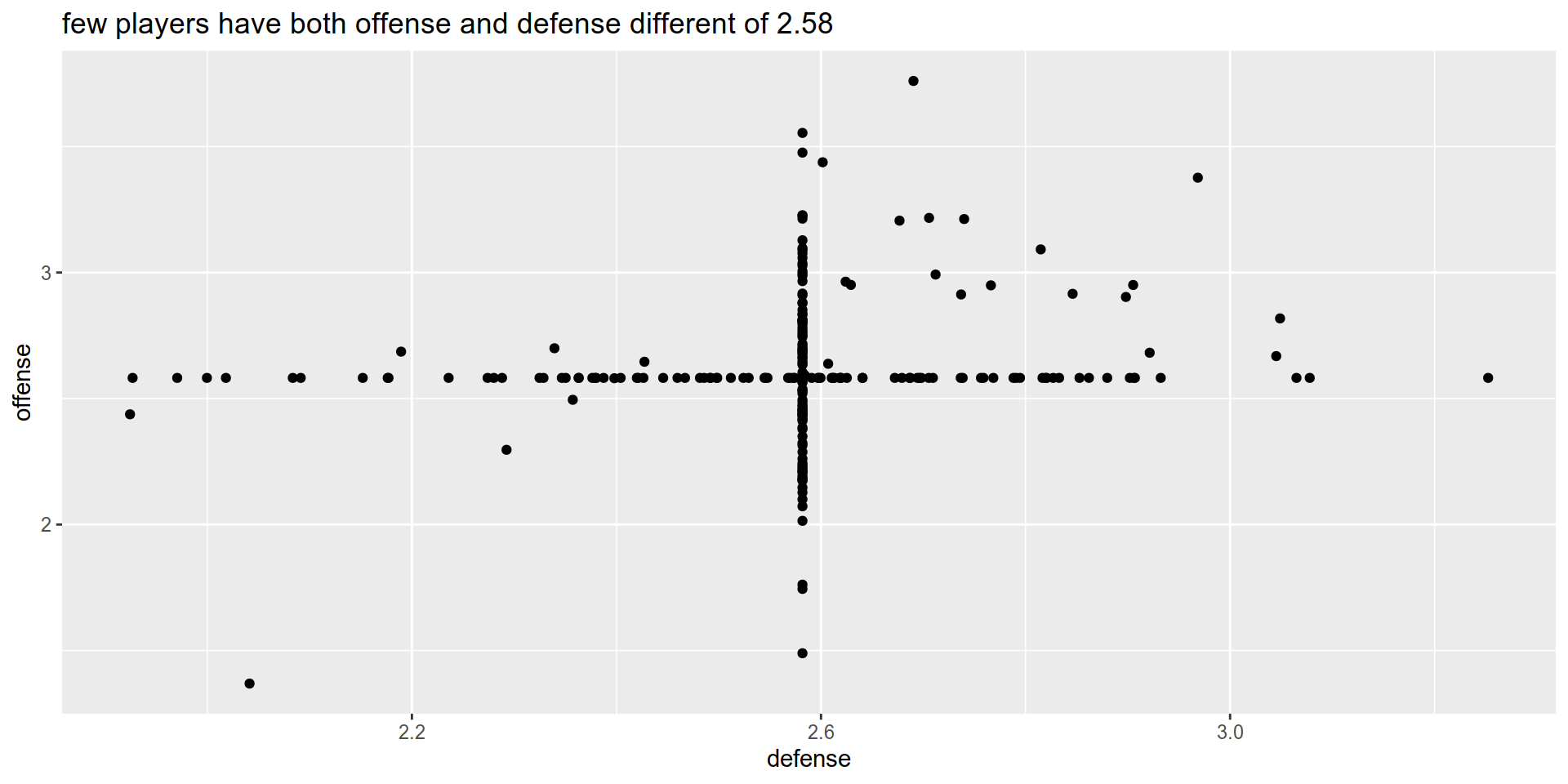
So this kinda worked. Results aren’t too different from expectations, with Crosby and Kucherov getting pretty good results. There is one issue that remains: everyone should be getting a specific value for offense and defense, but the model has allocated the “average” value for offense or defense to a very high number of players.
I tried increasing the number of trees ( to 50 000!) and reducing the learning rate to allow the model to better segment “average looking players”, but the problem isnt solved. I probably need more data, so a solution might involve looking at more seasons looking at shots (controlling for quality) instead of goals.
So, what do you guys think?