Tweedie vs Poisson * Gamma
I’m building my first tweedie model, and I’m finally trying the {recipes} package.
We will try to predict the pure premium of car insurance policy. This can be done directly with a tweedie model, or by multiplying two separates models: a frequency (Poisson) and a severity (Gamma) model. We wil be using “lift charts” and “double lift charts” to evaluate the model performance .
Here’s is the plan:
- Pre-process the train and test data using
recipes.
- Estimate the pure premium directly using a Tweedie model (93% of
claimcst0values are 0$, the others are the claims dollar amount).
- Estimate the frequency of claims using a Poisson model (93% of values
clmvalues are 0, the other are equal to 1). - Estimate the severity of claims using a Gamma model (estimate the
claimcst0value for the 7% that is above 0$)
- All three models are estimated using a GLM and a GBM approach.
- Models are compared using three approaches :
- Normalized Gini Index,
- Lift charts,
- Double-lift charts.
More details about these charts here. What I call “lift chart” is named “simple quantile plots” in the pdf.
tl;dr: recipes is AWESOME. Also, both glm and xgboost models all perform poorly. I made a new post using 6M observatiosn instead of 67k, and it helps.
Reasons I will come back to this post for code snippets:
* the rsample, yardstick and recipes packages are used for pre-processing data. I don’t know everything it can do, but I found ot is very useful to prevent leaking data from the test set into the train set, and to generate all the models to impute missing datas.
* My double-lift chart generation function disloc() and lift-chart generation function get_lift_chart() finally look good.
* This is my first tweedie, both using glm (package statmod) and xgboost.
TODO: learn tuner to find the best xgboost hyperparameters and tweedie parameters.
Libraries
The data comes from the insuranceData package, described below in the data section.
Data wrangling and plot is done using the tidyverse and patchwork, as usual.
The statmod library is required to evaluate tweedie models using GLM.
modelris used for the add_predictions() function.
broom::tidy()is used to get GLM coefficients in table format,
xgboost is used to evaluate the gradient boosting model.
tictoc::tic() and tictoc::toc() are used to measure evaluation time.
Claus Wilke’s cowplot::theme_cowplot(), dviz.supp::theme_dviz_hgrid() and colorblindr::scale_color_OkabeIto() are used for to make my plots look better
MLmetrics::NormalizedGini for normalized gini coefficient.
# https://www.cybaea.net/Journal/2012/03/13/R-code-for-Chapter-2-of-Non_Life-Insurance-Pricing-with-GLM/
library(insuranceData) # for  dataCar  insurance data
library(tidyverse)  # pour la manipulation de données
library(statmod) #pour glm(family = tweedie)
library(modelr) # pour add_predictions()
library(broom) # pour afficher les coefficients
library(tidymodels)
library(xgboost)
library(tictoc)
library(dviz.supp) # devtools::install_github("clauswilke/dviz.supp")
library(colorblindr)  # devtools::install_github("clauswilke/colorblindr")
library(patchwork)
library(rsample)
library(yardstick)
library(recipes)
library(MLmetrics) # for normalized gini
Data
The dataCar data from the insuranceData package. It contains 67 856 one-year vehicle insurance policies taken out in 2004 or 2005. It originally came with the book Generalized Linear Models for Insurance Data (2008).
The exposure variable represents the “number of year of exposure” and is used as the offset variable. It is bounded between 0 and 1.
Finally, the independent variables are as follow:
veh_value, the vehicle value in tens of thousand of dollars,
veh_body, y vehicle body, coded as BUS CONVT COUPE HBACK HDTOP MCARA MIBUS PANVN RDSTR SEDAN STNWG TRUCK UTE,
veh_age, 1 (youngest), 2, 3, 4,
gender, a factor with levels F M,
areaa factor with levels A B C D E F,
agecat1 (youngest), 2, 3, 4, 5, 6
The dollar amount of the claims is claimcst0. We will divide it by the exposure to obtain annual_loss which is the pure annual premium.
For the frequency (Poisosn) model, we will model clm (0 or 1) because the cost variables (claimcst0) represents the total cost, if you have multiple claims (numclaims>1).
Pre-process the data using recipe
I’ve used a few tutorials and vignettes, including the following two:
https://cran.r-project.org/web/packages/recipes/vignettes/Simple_Example.html https://www.andrewaage.com/post/a-simple-solution-to-a-kaggle-competition-using-xgboost-and-recipes/
I honestly havent done that much reading, but here is why I have adopted recipes. :
* create dummies for xgboost in 1 line of code,
* trainn knn models to impute all missing predictors in 1 line of code,
* combine super rare categories into “other” in 1 line of code, (not done here, but all is needed is step_knnimpute(all_predictors()))
All while making sure that you don’t leak any test data into your train data. What’s not to like?
data(dataCar)

# claimcst0 = claim amount (0 if no claim)
# clm = 0 or 1 = has a claim yes/ no
#  numclaims = number of claims  0 , 1 ,2 ,3 or 4).
# we use clm because the corresponding dollar amount is for all claims combined.
mydb <- dataCar %>% select(clm, claimcst0, exposure, veh_value, veh_body,
                           veh_age, gender, area, agecat) %>%
  mutate(annual_loss = claimcst0 / exposure)

set.seed(42)

split <- rsample::initial_split(mydb, prop = 0.8)
train <- rsample::training(split)
test <- rsample::testing(split)

rec <-  recipes::recipe(train %>% select(annual_loss, clm, claimcst0,  exposure, veh_value,veh_body, veh_age, gender,area,agecat)) %>%
  recipes::update_role(everything(), new_role = "predictor") %>%
  recipes::update_role(annual_loss, new_role = "outcome") %>%
  recipes::update_role(clm, new_role = "outcome") %>%
  recipes::update_role(claimcst0, new_role = "outcome") %>%
  recipes::update_role(exposure, new_role = "case weight") %>%
  recipes::step_zv(recipes::all_predictors()) %>%   # remove variable with all equal values
  recipes::step_other(recipes::all_predictors(), threshold = 0.01)  %>%       # combine categories with less than 1% of observation
  recipes::step_dummy(recipes::all_nominal())  %>% # convert to dummy for xgboost use
  check_missing(all_predictors()) ## break the bake function if any of the checked columns contains NA value

# Prepare the recipe and use juice/bake to get the data!
prepped_rec <- prep(rec)
train <- juice(prepped_rec)
test <- bake(prepped_rec, new_data = test)
GLMs
Poisson model (frequency)
We model the presence of a claim (clm) and use the log(exposure) as an offset.
poisson_fit <-
  glm(clm ~ . -annual_loss -exposure -claimcst0 ,
      family = poisson(link = "log"),
      offset = log(exposure),
      data = train)

#broom::tidy(poisson_fit)
summary(poisson_fit)
##
## Call:
## glm(formula = clm ~ . - annual_loss - exposure - claimcst0, family = poisson(link = "log"),
##     data = train, offset = log(exposure))
##
## Deviance Residuals:
##     Min       1Q   Median       3Q      Max
## -0.7375  -0.4364  -0.3346  -0.2142   3.5503
##
## Coefficients:
##                  Estimate Std. Error z value Pr(>|z|)
## (Intercept)     -1.054539   0.235626  -4.475 7.62e-06 ***
## veh_age         -0.076200   0.015751  -4.838 1.31e-06 ***
## agecat          -0.085522   0.011886  -7.195 6.24e-13 ***
## veh_value_other  0.080809   0.186824   0.433 0.665348
## veh_body_HBACK  -0.516787   0.135851  -3.804 0.000142 ***
## veh_body_HDTOP  -0.284150   0.163919  -1.733 0.083012 .
## veh_body_MIBUS  -0.564570   0.220348  -2.562 0.010402 *
## veh_body_PANVN  -0.400556   0.193340  -2.072 0.038287 *
## veh_body_SEDAN  -0.479023   0.135038  -3.547 0.000389 ***
## veh_body_STNWG  -0.399992   0.136005  -2.941 0.003271 **
## veh_body_TRUCK  -0.509168   0.168834  -3.016 0.002563 **
## veh_body_UTE    -0.669788   0.150302  -4.456 8.34e-06 ***
## veh_body_other  -0.103584   0.254960  -0.406 0.684540
## gender_M        -0.003482   0.034668  -0.100 0.919994
## area_B           0.064939   0.049370   1.315 0.188387
## area_C           0.018744   0.045098   0.416 0.677686
## area_D          -0.122612   0.061803  -1.984 0.047266 *
## area_E          -0.008238   0.066679  -0.124 0.901675
## area_F          -0.001512   0.078559  -0.019 0.984646
## ---
## Signif. codes:  0 '***' 0.001 '**' 0.01 '*' 0.05 '.' 0.1 ' ' 1
##
## (Dispersion parameter for poisson family taken to be 1)
##
##     Null deviance: 19004  on 54284  degrees of freedom
## Residual deviance: 18885  on 54266  degrees of freedom
## AIC: 26279
##
## Number of Fisher Scoring iterations: 6
Gamma model
For the 7% of policies with a claim, we model the dollar amount of claims (claimcst0)
gamma_fit <-
  glm(claimcst0 ~ . -annual_loss -exposure -clm ,
      data = train %>% filter( claimcst0 > 0),
      family = Gamma("log"))

#broom::tidy(gamma_fit)
summary(gamma_fit)
##
## Call:
## glm(formula = claimcst0 ~ . - annual_loss - exposure - clm, family = Gamma("log"),
##     data = train %>% filter(claimcst0 > 0))
##
## Deviance Residuals:
##     Min       1Q   Median       3Q      Max
## -1.9490  -1.3477  -0.7828   0.0977   6.9485
##
## Coefficients:
##                  Estimate Std. Error t value Pr(>|t|)
## (Intercept)      7.987519   0.391035  20.427  < 2e-16 ***
## veh_age          0.049425   0.026406   1.872 0.061329 .
## agecat          -0.052324   0.019640  -2.664 0.007752 **
## veh_value_other -0.141215   0.310703  -0.455 0.649494
## veh_body_HBACK  -0.271797   0.225970  -1.203 0.229131
## veh_body_HDTOP  -0.405127   0.272327  -1.488 0.136930
## veh_body_MIBUS  -0.331422   0.366175  -0.905 0.365476
## veh_body_PANVN  -0.191639   0.321404  -0.596 0.551042
## veh_body_SEDAN  -0.442009   0.224734  -1.967 0.049281 *
## veh_body_STNWG  -0.508804   0.226379  -2.248 0.024662 *
## veh_body_TRUCK  -0.236181   0.281025  -0.840 0.400723
## veh_body_UTE    -0.290821   0.250266  -1.162 0.245291
## veh_body_other  -0.930757   0.423793  -2.196 0.028136 *
## gender_M         0.151658   0.057777   2.625 0.008704 **
## area_B           0.009213   0.082098   0.112 0.910657
## area_C           0.086454   0.075065   1.152 0.249507
## area_D          -0.018480   0.103047  -0.179 0.857682
## area_E           0.247247   0.111179   2.224 0.026219 *
## area_F           0.432186   0.130822   3.304 0.000964 ***
## ---
## Signif. codes:  0 '***' 0.001 '**' 0.01 '*' 0.05 '.' 0.1 ' ' 1
##
## (Dispersion parameter for Gamma family taken to be 2.757837)
##
##     Null deviance: 5705.3  on 3677  degrees of freedom
## Residual deviance: 5556.3  on 3659  degrees of freedom
## AIC: 62848
##
## Number of Fisher Scoring iterations: 7
XGBoost
XGBoost Tweedie Model
xgtrain_tweedie <- xgb.DMatrix(as.matrix(train %>% select(-annual_loss ,-clm, - claimcst0, -exposure )),
                               label = train$annual_loss,
                               weight = train$exposure
)


xgtest_tweedie <- xgb.DMatrix(as.matrix(test %>% select(-annual_loss ,-clm, - claimcst0, -exposure )),
                              label = test$annual_loss,
                              weight = test$exposure
)


params <-list(
  booster = "gbtree",
  objective = 'reg:tweedie',
  eval_metric = "tweedie-nloglik@1.1",
  tweedie_variance_power = 1.1,
  gamma = 0,
  max_depth = 4,
  eta = 0.01,
  min_child_weight = 3,
  subsample = 0.8,
  colsample_bytree = 0.8,
  tree_method = "hist"
)

xgcv_tweedie <- xgb.cv(
  params = params,
  data = xgtrain_tweedie,
  nround = 1000,
  nfold=  5,
  showsd = TRUE,
  early_stopping_rounds = 50,
  verbose = 0)

xgcv_tweedie$best_iteration
## [1] 319


# xgb.cv doesnt ouput any model -- we need a model to predict test dataset
xgmodel_tweedie <- xgboost::xgb.train(
  data = xgtrain_tweedie,
  params = params,
  nrounds = xgcv_tweedie$best_iteration,
  nthread = parallel::detectCores() - 1
)
XGBoost Poisson model
xgtrain_poisson <- xgb.DMatrix(as.matrix(train %>% select(-annual_loss ,-clm, - claimcst0, -exposure )),
                               label = train$clm
)


xgtest_poisson <- xgb.DMatrix(as.matrix(test %>% select(-annual_loss ,-clm, - claimcst0, -exposure )),
                              label = test$clm
)

setinfo(xgtrain_poisson,"base_margin",
        train %>% pull(exposure) %>% log() )
## [1] TRUE

setinfo(xgtest_poisson,"base_margin",
        train %>% pull(exposure) %>% log() )
## [1] TRUE

params <-list(
  booster = "gbtree",
  objective = 'count:poisson',
  eval_metric = "poisson-nloglik",
  gamma = 0,
  max_depth = 4,
  eta = 0.05,
  min_child_weight = 3,
  subsample = 0.8,
  colsample_bytree = 0.8,
  tree_method = "hist"
)

xgcv_poisson <- xgb.cv(
  params = params,
  data = xgtrain_poisson,
  nround = 1000,
  nfold=  5,
  showsd = TRUE,
  early_stopping_rounds = 50,
  verbose = 0)

xgcv_poisson$best_iteration
## [1] 212


# xgb.cv doesnt ouput any model -- we need a model to predict test dataset
xgmodel_poisson <- xgboost::xgb.train(
  data = xgtrain_poisson,
  params = params,
  nrounds = xgcv_poisson$best_iteration,
  nthread = parallel::detectCores() - 1
)
XGBoost Gamma model
Gamma model is only train on policy with claims
xgtrain_gamma <- xgb.DMatrix(as.matrix(train %>% filter(claimcst0 > 0) %>%select(-annual_loss ,-clm, - claimcst0, -exposure )),
                             label = train %>% filter(claimcst0 > 0) %>% pull(claimcst0)
)

xgtest_gamma <- xgb.DMatrix(as.matrix(test %>% select(-annual_loss ,-clm, - claimcst0, -exposure )),
                            label = test$claimcst0
)

params <-list(
  booster = "gbtree",
  objective = 'reg:gamma',
  gamma = 0,
  max_depth = 4,
  eta = 0.05,
  min_child_weight = 3,
  subsample = 0.8,
  colsample_bytree = 0.8,
  tree_method = "hist"
)

xgcv_gamma <- xgb.cv(
  params = params,
  data = xgtrain_gamma,
  nround = 1000,
  nfold=  5,
  showsd = TRUE,
  early_stopping_rounds = 50,
  verbose = 0)

xgcv_gamma$best_iteration
## [1] 222


# xgb.cv doesnt ouput any model -- we need a model to predict test dataset
xgmodel_gamma <- xgboost::xgb.train(
  data = xgtrain_gamma,
  params = params,
  nrounds = xgcv_gamma$best_iteration,
  nthread = parallel::detectCores() - 1
)
Functions lift & double lift
# double lift charts
#' @title disloc()
#'
#' @description Cette fonction crée un tableau et une double lift chart
#' @param data data.frame  source
#' @param pred1 prediction of first model
#' @param pred1 prediction of second model
#' @param expo exposure var
#' @param obs observed result
#' @param nb nombre de quantils créés
#' @param obs_lab Label pour la valeur observée dans le graphique
#' @param pred1_lab Label pour la première prédiction dans le graphique
#' @param pred2_lab Label pour la deuxième prédiction dans le graphique
#' @param x_label Label pour la valeur réalisée dans le graphique
#' @param y_label Label pour la valeur réalisée dans le graphique
#' @param y_format Fonction utilisée pour formater l'axe des y dans le graphique (par exemple percent_format() ou dollar_format() du package scales)
#' @export

disloc <- function(data, pred1, pred2, expo, obs, nb = 10,
                   obs_lab = "",
                   pred1_lab = "", pred2_lab = "",
                   x_label = "",
                   y_label= "sinistralité",
                   y_format = scales::number_format(accuracy = 1,  big.mark = " ", decimal.mark = ",")
) {
  # obligé de mettre les variables dans un enquo pour pouvoir les utiliser dans dplyr

  pred1_var <- enquo(pred1)
  pred2_var <- enquo(pred2)
  expo_var <- enquo(expo)
  obs_var <- enquo(obs)


  pred1_name <- quo_name(pred1_var)
  pred2_name <- quo_name(pred2_var)
  obs_name <- quo_name(obs_var)


  if (pred1_lab =="") {pred1_lab <- pred1_name}
  if (pred2_lab =="") {pred2_lab <- pred2_name}
  if (obs_lab =="") {obs_lab <- obs_name}

  if (x_label == ""){ x_label <- paste0("ratio entre les prédictions ", pred1_lab, " / ", pred2_lab)}

  # création de la comparaison entre les deux pred
  dd <- data %>%
    mutate(ratio = !!pred1_var / !!pred2_var) %>%
    filter(!!expo_var > 0) %>%
    drop_na()

  # constitution des buckets de poids égaux
  dd <- dd %>% add_equal_weight_group(
    sort_by = ratio,
    expo = !!expo_var,
    group_variable_name = "groupe",
    nb = nb
  )

  # comparaison sur ces buckets
  dd <- full_join(
    dd %>% group_by(groupe) %>%
      summarise(
        ratio_moyen = mean(ratio),
        ratio_min = min(ratio),
        ratio_max = max(ratio)
      ),
    dd %>% group_by(groupe) %>%
      summarise_at(
        funs(sum(.) / sum(!!expo_var)),
        .vars = vars(!!obs_var, !!pred1_var, !!pred2_var)
      ) %>%
      ungroup,
    by = "groupe"
  )

  # création des labels
  dd <- dd %>%
    mutate(labs = paste0("[", round(ratio_min, 2), ", ", round(ratio_max, 2), "]"))

  # graphe
  plotdata <-
    dd %>%
    gather(key, variable, !!obs_var, !!pred1_var, !!pred2_var) %>%
    ## Pas optimal mais je ne trouve pas mieux...
    mutate(key = case_when(
      key == obs_name ~ obs_lab,
      key == pred1_name ~ pred1_lab,
      key == pred2_name ~ pred2_lab
    )) %>%
    mutate(key = factor(key, levels = c(obs_lab, pred1_lab, pred2_lab), ordered = TRUE))

  pl <- plotdata %>%
    ggplot(aes(ratio_moyen, variable, color = key, linetype = key)) +
    cowplot::theme_cowplot() +
    cowplot::background_grid()+
    colorblindr::scale_color_OkabeIto( ) +

    scale_x_continuous(breaks = scales::pretty_breaks())+
    geom_line() +
    geom_point() +
    scale_x_continuous(breaks = dd$ratio_moyen, labels = dd$labs) +
    scale_y_continuous(breaks = scales::pretty_breaks() )+
    labs(
      x = x_label,
      y = y_label
    )+
    theme(axis.text.x = element_text(angle = 30, hjust = 1, vjust = 1)) #+


  # écart au réalisé, pondéré
  ecart <- dd %>%
    mutate(poids = abs(1 - ratio_moyen)) %>%
    summarise_at(
      vars(!!pred1_var, !!pred2_var),
      funs(weighted.mean((. - !!obs_var)^2, w = poids) %>% sqrt())
    ) %>% summarise(ratio_distance = !!pred2_var / !!pred1_var) %>%
    as.numeric()

  list(
    graphe = pl,
    ecart = ecart,
    tableau = dd
  )
}

#' @title add_equal_weight_group()
#'
#' @description Cette fonction crée des groupe (quantiles) avec le nombre nombre total d'exposition.
#' @param table data.frame  source
#' @param sort_by Variable utilisée pour trier les observations.
#' @param expo Exposition (utilisée pour créer des quantiles de la même taille.  Si NULL, l'exposition est égale pour toutes les observations) (Défault = NULL).
#' @param nb Nombre de quantiles crées (défaut = 10)
#' @param group_variable_name Nom de la variable de groupes créée
#' @export


add_equal_weight_group <- function(table, sort_by, expo = NULL, group_variable_name = "groupe", nb = 10) {
  sort_by_var <- enquo(sort_by)
  groupe_variable_name_var <- enquo(group_variable_name)

  if (!(missing(expo))){ # https://stackoverflow.com/questions/48504942/testing-a-function-that-uses-enquo-for-a-null-parameter

    expo_var <- enquo(expo)

    total <- table %>% pull(!!expo_var) %>% sum
    br <- seq(0, total, length.out = nb + 1) %>% head(-1) %>% c(Inf) %>% unique
    table %>%
      arrange(!!sort_by_var) %>%
      mutate(cumExpo = cumsum(!!expo_var)) %>%
      mutate(!!group_variable_name := cut(cumExpo, breaks = br, ordered_result = TRUE, include.lowest = TRUE) %>% as.numeric) %>%
      select(-cumExpo)
  } else {
    total <- nrow(table)
    br <- seq(0, total, length.out = nb + 1) %>% head(-1) %>% c(Inf) %>% unique
    table %>%
      arrange(!!sort_by_var) %>%
      mutate(cumExpo = row_number()) %>%
      mutate(!!group_variable_name := cut(cumExpo, breaks = br, ordered_result = TRUE, include.lowest = TRUE) %>% as.numeric) %>%
      select(-cumExpo)
  }
}

get_lift_chart_data <- function(
  data,
  sort_by,
  pred,
  expo,
  obs,
  nb = 10) {

  pred_var <- enquo(pred)
  sort_by_var <- enquo(sort_by)
  expo_var <- enquo(expo)
  obs_var <- enquo(obs)


  pred_name <- quo_name(pred_var)
  sort_by_name <- quo_name(sort_by_var)
  obs_name <- quo_name(obs_var)

  # constitution des buckets de poids égaux
  dd <- data %>% add_equal_weight_group(
    sort_by = !!sort_by_var,
    expo = !!expo_var,
    group_variable_name = "groupe",
    nb = nb
  )

  # comparaison sur ces buckets
  dd <- full_join(
    dd %>%
      group_by(groupe) %>%
      summarise(
        exposure = sum(!!expo_var),
        sort_by_moyen = mean(!!sort_by_var),
        sort_by_min = min(!!sort_by_var),
        sort_by_max = max(!!sort_by_var)
      ) %>%
      ungroup(),
    dd %>%
      group_by(groupe) %>%
      summarise_at(
        funs(sum(.) / sum(!!expo_var)),
        .vars = vars(!!obs_var, !!pred_var)
      ) %>%
      ungroup,
    by = "groupe"
  )

  # création des labels
  dd <- dd %>%
    mutate(labs = paste0("[", round(sort_by_min, 2), ", ", round(sort_by_max, 2), "]"))

}

get_lift_chart <- function(data,
                           sort_by,
                           pred,
                           expo,
                           obs,
                           nb){

  pred_var <- enquo(pred)
  sort_by_var <- enquo(sort_by)
  expo_var <- enquo(expo)
  obs_var <- enquo(obs)

  lift_data <- get_lift_chart_data(
    data = data,
    sort_by = !!sort_by_var,
    pred = !!pred_var,
    expo = !!expo_var,
    obs = !!obs_var,
    nb = 10)

  p1 <- lift_data %>%
    mutate(groupe = as.factor(groupe)) %>%
    select(groupe, labs, !!pred_var, !!obs_var) %>%
    gather(key = type, value = average, !!pred_var, !!obs_var)  %>%
    ggplot(aes(x= groupe, y = average, color =type, group = type)) +
    geom_line() +
    geom_point()+
    cowplot::theme_half_open() +
    cowplot::background_grid() +
    colorblindr::scale_color_OkabeIto( ) +
    # scale_y_continuous(
    #   breaks  = scales::pretty_breaks()
    # )+
    theme(
      legend.position = c(0.1, 0.8),
      axis.title.x=element_blank(),
      axis.text.x=element_blank(),
      axis.ticks.x=element_blank()
    )

  p2 <- lift_data %>%
    mutate(groupe = as.factor(groupe)) %>%
    select(groupe, labs, exposure) %>%
    ggplot(aes(x= groupe, y = exposure)) +
    geom_col() +
    cowplot::theme_half_open() +
    cowplot::background_grid() +
    colorblindr::scale_color_OkabeIto( )# +
    # scale_y_continuous(
    #   expand = c(0,0),
    #   breaks  = scales::breaks_pretty(3)
    # )

  return(p1 / p2 +   plot_layout(heights = c(3, 1)))
}
Results
Add predictions to the test dataset.
Quick check: the means for predictions of frequency and total cost don’t appear to be way off
test_w_preds <- test %>%
  add_predictions("pred_annual_loss_glm", model = tweedie_fit, type = "response") %>%
  mutate(pred_loss_glm = pred_annual_loss_glm * exposure) %>%
  add_predictions("pred_poisson_glm", model = poisson_fit, type = "response") %>%
  add_predictions("pred_gamma_glm", model = gamma_fit, type = "response")  %>%
  mutate(pred_frequency_severity_glm = pred_poisson_glm * pred_gamma_glm,
         pred_annual_loss_xgboost = predict(xgmodel_tweedie, xgtest_tweedie),
         pred_loss_xgboost = pred_annual_loss_xgboost * exposure,
         pred_poisson_xgboost =  predict(xgmodel_poisson, xgtest_poisson),
         pred_gamma_xgboost =  predict(xgmodel_gamma, xgtest_gamma),
         pred_frequency_severity_xgboost = pred_poisson_xgboost * pred_gamma_xgboost,
         pred_annual_freq_glm = pred_poisson_glm / exposure,
         pred_annual_freq_xgboost = pred_poisson_xgboost / exposure,)


test_w_preds %>%
  select(claimcst0, pred_loss_glm, pred_frequency_severity_glm, pred_loss_xgboost, pred_frequency_severity_xgboost,
         clm, pred_poisson_glm, pred_poisson_xgboost) %>%
  skimr::skim() %>%
knitr::kable(digits = 3L)| skim_type | skim_variable | n_missing | complete_rate | numeric.mean | numeric.sd | numeric.p0 | numeric.p25 | numeric.p50 | numeric.p75 | numeric.p100 | numeric.hist |
|---|---|---|---|---|---|---|---|---|---|---|---|
| numeric | claimcst0 | 0 | 1 | 161.098 | 1283.589 | 0.000 | 0.000 | 0.000 | 0.000 | 55922.130 | ▇▁▁▁▁ |
| numeric | pred_loss_glm | 0 | 1 | 131.153 | 94.004 | 0.382 | 56.520 | 117.134 | 187.708 | 786.876 | ▇▃▁▁▁ |
| numeric | pred_frequency_severity_glm | 0 | 1 | 131.292 | 94.274 | 0.379 | 56.559 | 117.243 | 187.708 | 770.042 | ▇▃▁▁▁ |
| numeric | pred_loss_xgboost | 0 | 1 | 120.634 | 98.135 | 0.278 | 51.604 | 106.094 | 171.248 | 3875.319 | ▇▁▁▁▁ |
| numeric | pred_frequency_severity_xgboost | 0 | 1 | 130.627 | 34.040 | 43.804 | 108.232 | 128.887 | 145.492 | 520.413 | ▇▃▁▁▁ |
| numeric | clm | 0 | 1 | 0.070 | 0.255 | 0.000 | 0.000 | 0.000 | 0.000 | 1.000 | ▇▁▁▁▁ |
| numeric | pred_poisson_glm | 0 | 1 | 0.067 | 0.044 | 0.000 | 0.030 | 0.063 | 0.100 | 0.286 | ▇▆▃▁▁ |
| numeric | pred_poisson_xgboost | 0 | 1 | 0.075 | 0.013 | 0.036 | 0.066 | 0.075 | 0.082 | 0.165 | ▂▇▂▁▁ |
Normalized Gini
The GLM model systematically perform better than the XGB models.
The XGB combination of Frequency and Severity models has a Normalized Gini 4x smaller than it’s GLM counterpart.
We will really need to do this exercise again with a larger dataset.
Poisson_GLM = MLmetrics::NormalizedGini(test_w_preds$clm, test_w_preds$pred_poisson_glm)
Poisson_XGB = MLmetrics::NormalizedGini(test_w_preds$clm, test_w_preds$pred_poisson_xgboost)
Tweedie_GLM = MLmetrics::NormalizedGini(test_w_preds$claimcst0, test_w_preds$pred_loss_glm)
Tweedie_XGB = MLmetrics::NormalizedGini(test_w_preds$claimcst0, test_w_preds$pred_loss_xgboost)
FreqSev_GLM = MLmetrics::NormalizedGini(test_w_preds$claimcst0, test_w_preds$pred_frequency_severity_glm)
FreqSev_XGB = MLmetrics::NormalizedGini(test_w_preds$claimcst0, test_w_preds$pred_frequency_severity_xgboost    )


tibble(Poisson_GLM,
       Poisson_XGB,
       Tweedie_GLM,
       Tweedie_XGB,
       FreqSev_GLM,
       FreqSev_XGB) %>%
  gather(key = model, value = NormalizedGini) %>%
knitr::kable(digits = 3L)| model | NormalizedGini |
|---|---|
| Poisson_GLM | 0.036 |
| Poisson_XGB | 0.018 |
| Tweedie_GLM | 0.041 |
| Tweedie_XGB | 0.042 |
| FreqSev_GLM | 0.041 |
| FreqSev_XGB | 0.026 |
Lift charts of select models
Tweedie GLM (pure premium)
get_lift_chart(
  data = test_w_preds,
  sort_by= pred_annual_loss_glm,
  pred = pred_loss_glm,
  obs = claimcst0,
  expo  = exposure )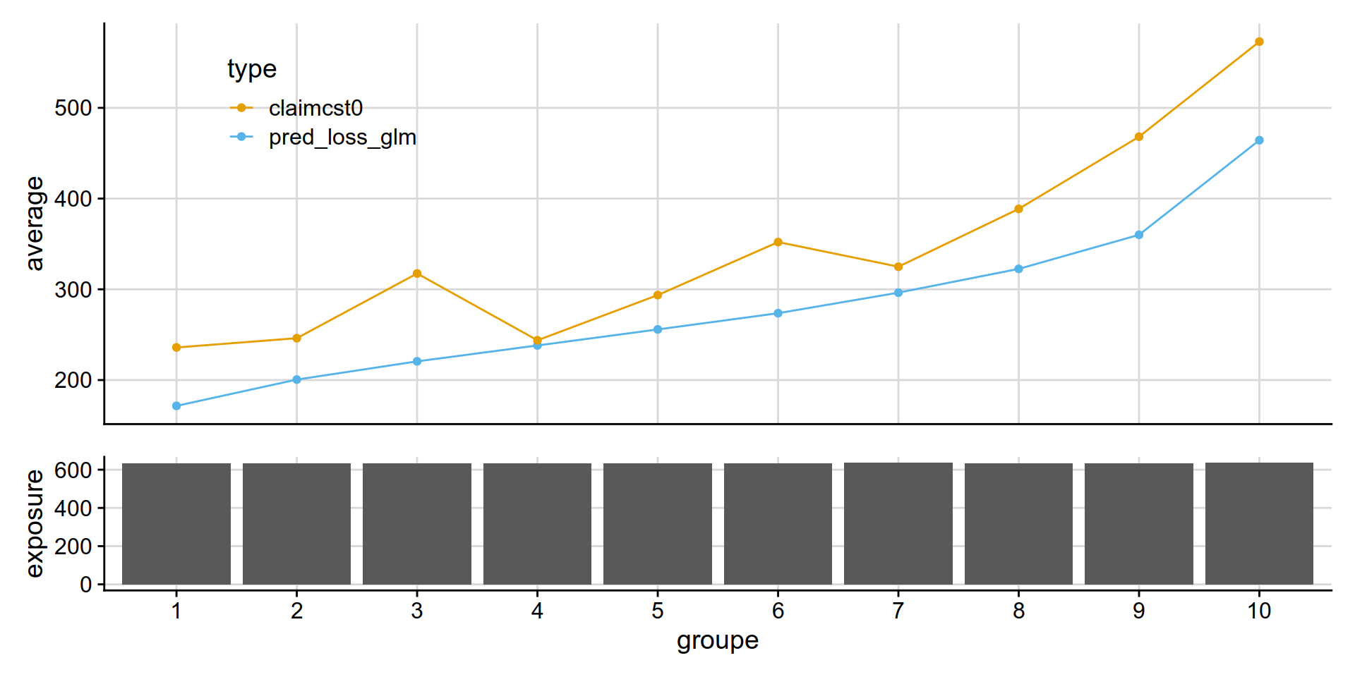
Tweedie XGBoost (pure premium)
get_lift_chart(
  data = test_w_preds,
  sort_by= pred_annual_loss_xgboost,
  pred = pred_loss_xgboost,
  obs = claimcst0,
  expo  = exposure )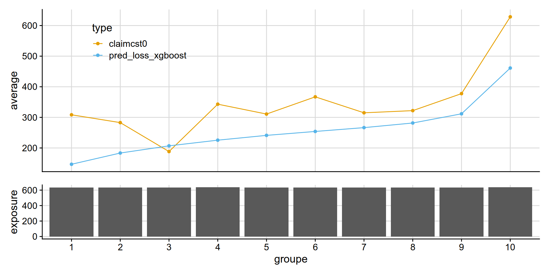
Poisson GLM (frequency)
get_lift_chart(
  data = test_w_preds,
  sort_by= pred_annual_freq_glm,
  pred = pred_poisson_glm,
  obs = clm,
  expo  = exposure )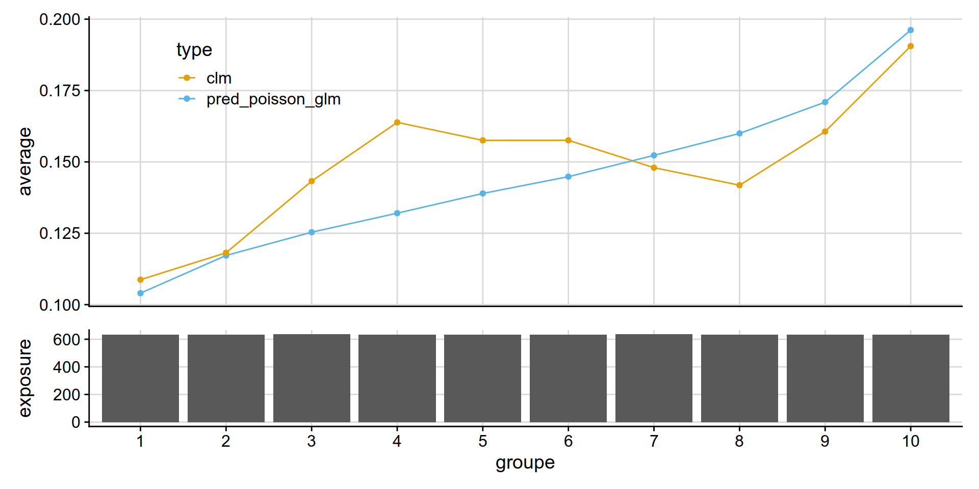
Poisson XGBoost (frequency)
get_lift_chart(
  data = test_w_preds,
  sort_by= pred_annual_freq_xgboost,
  pred = pred_poisson_xgboost,
  obs = clm,
  expo  = exposure )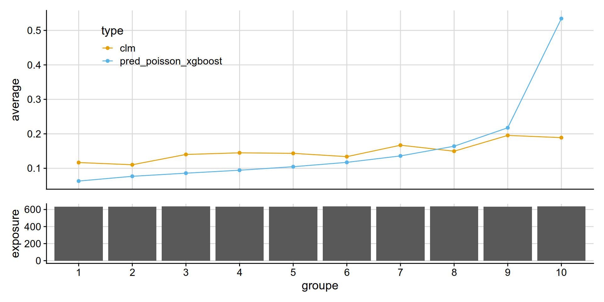
A test: extract individual plot from a patchwork object (it works!)
gaa2 <- get_lift_chart(
  data = test_w_preds,
  sort_by= pred_annual_freq_glm,
  pred = pred_poisson_glm,
  obs = clm,
  expo  = exposure )

gaa1 <- get_lift_chart(
  data = test_w_preds,
  sort_by= pred_annual_freq_xgboost,
  pred = pred_poisson_xgboost,
  obs = clm,
  expo  = exposure )

(gaa1[[1]] + gaa2[[1]]) /(gaa1[[2]] + gaa2[[2]])  +    plot_layout(heights = c(3, 1))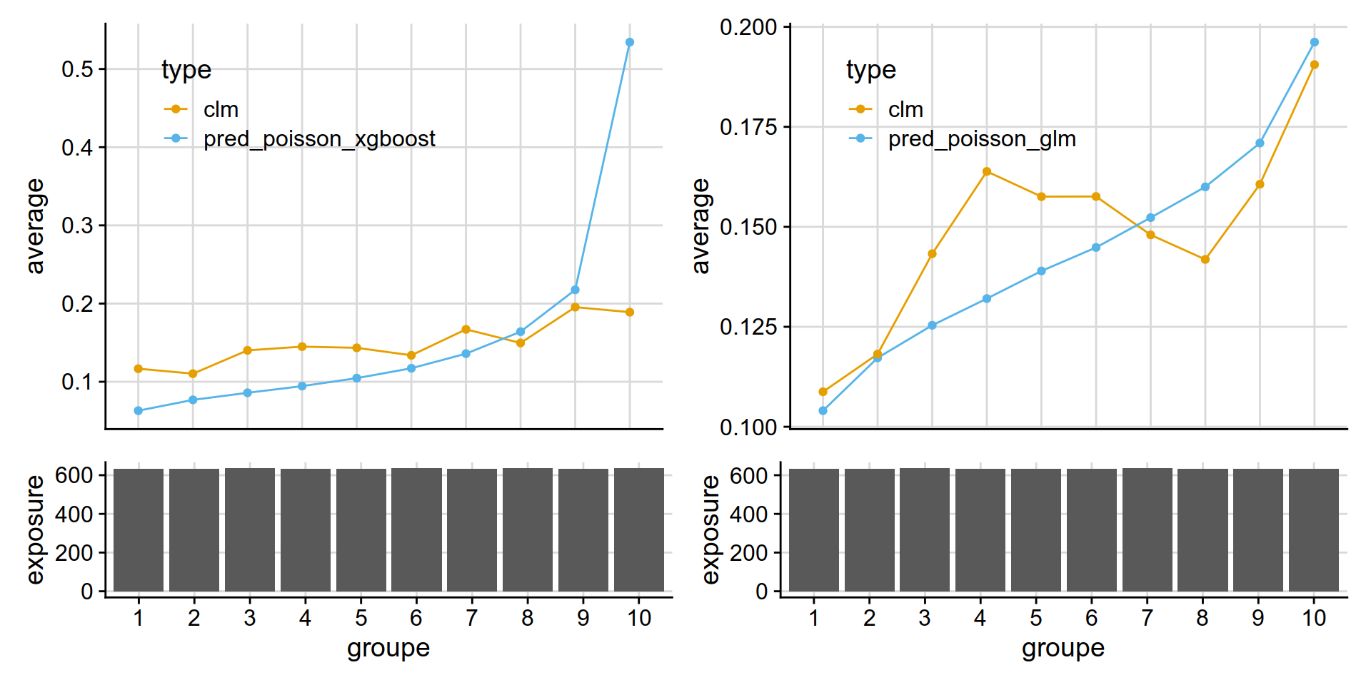
Double lift chart
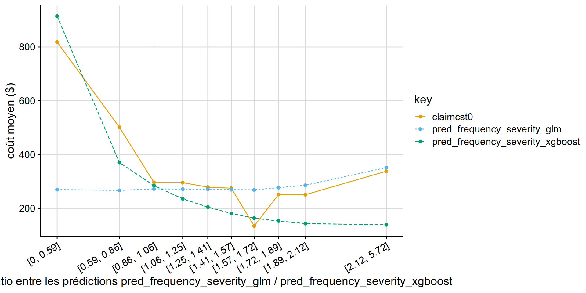
GLM Tweedie vs GLM Poisson * Gamma
GLM Tweedie ( power = 1.1) appears similar to than Poisson * Gamma .
disloc(data = test_w_preds,
       pred1 = pred_loss_glm,
       pred2 = pred_frequency_severity_glm,
       expo = exposure,
       obs = claimcst0 ,
       y_label = "coût moyen ($)"
) %>% .$graphe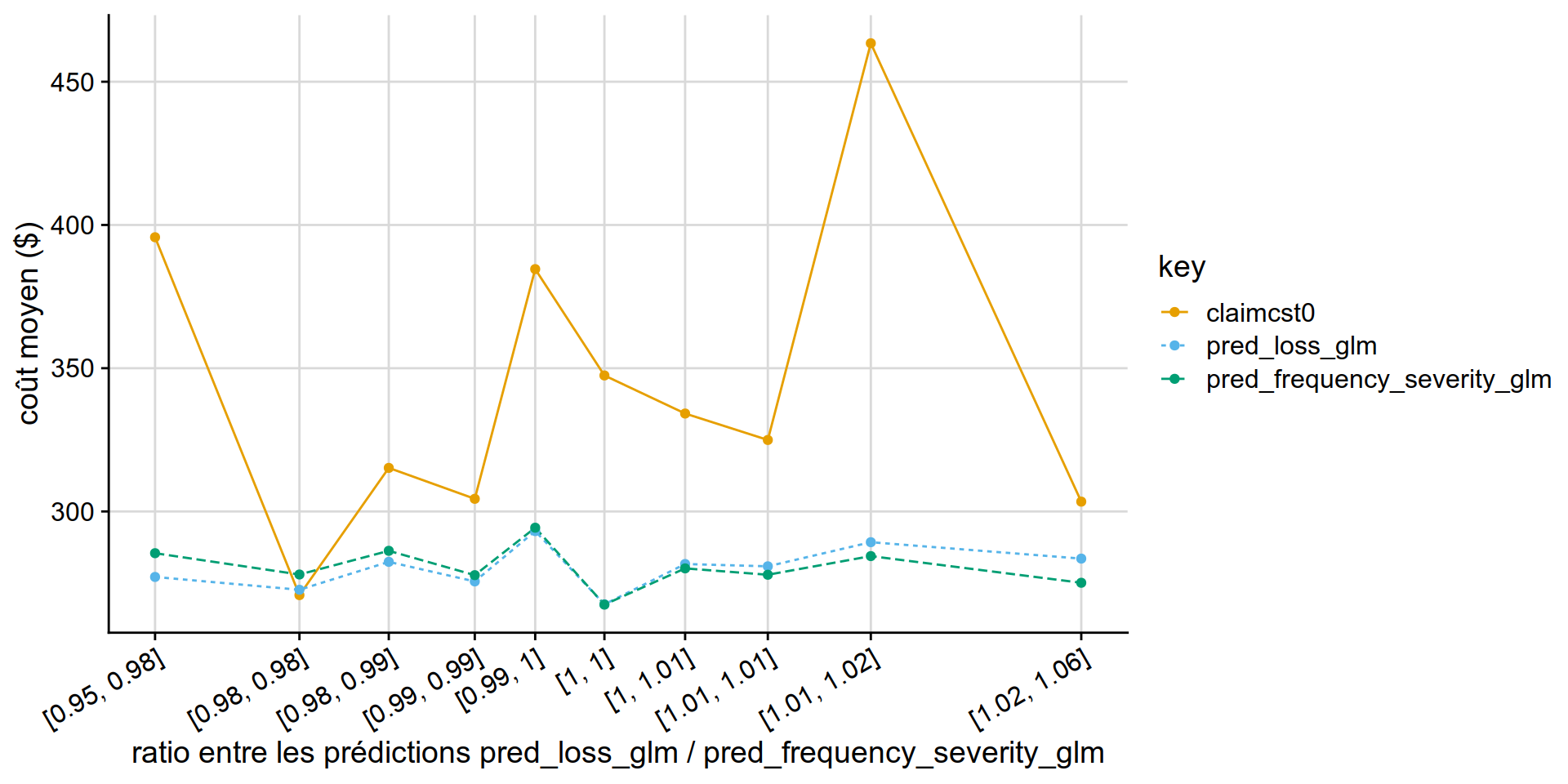
GLM Tweedie vs XGB Tweedie
Why is the xgboost tweedie doing so poorly vs GLM tweedie?
partial answer: xgboost is out of fold, glm can try to overfit.. but it really doesnt have that many variables to overfit on.
disloc(data = test_w_preds,
       pred1 = pred_loss_xgboost ,
       pred2 = pred_loss_glm,
       expo = exposure,
       obs = claimcst0 ,
       y_label = "coût moyen ($)"
) %>% .$graphe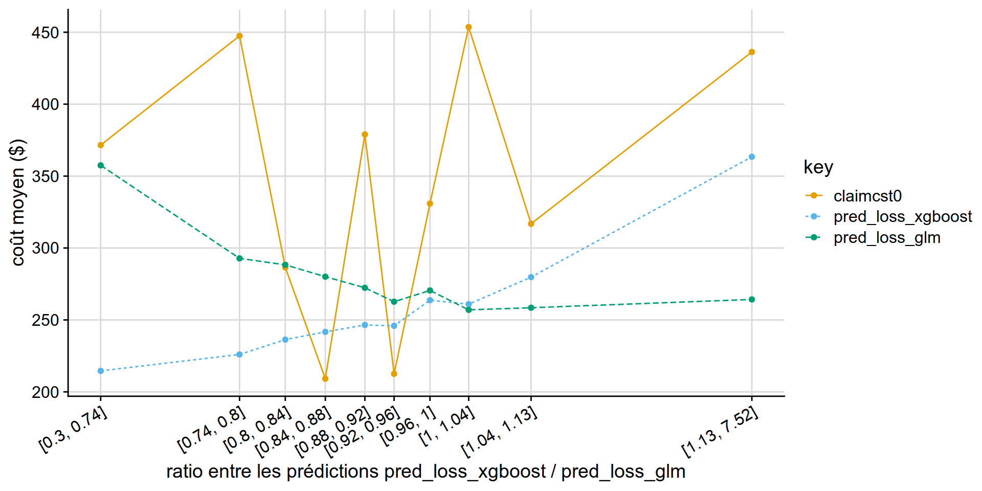
GLM PoissonGamma vs XGB PoissonGamma
disloc(data = test_w_preds,
       pred1 = pred_frequency_severity_glm,
       pred2 = pred_frequency_severity_xgboost,
       expo = exposure,
       obs = claimcst0 ,
       y_label = "coût moyen ($)"
) %>% .$graphe