
Animated map of ships, 1750-1799
I learned about the Climatological Database for the World’s Oceans (CLIWOC), a super cool database containing 287 116 days of ship log entries that have been digitized to better understand climate change.
Each record holds the date, the ship’s name, company and nationality, the latitude and longitude and a wealth of meteorological information.
Objective
I want to make an animated map with a bunch of moving ships because I can.
Data
I manually downloaded the CLIWOC 2.1 file in libreoffice calc format (*.ODS), then used libreoffice calc to save export it as a CSV. I made that CSV available on my AWS S3 bucket at https://blogsimoncoulombe.s3.amazonaws.com/cliwoc/cliwoc21.csv.
aws.s3::put_object(file = "/home/simon/git/adhoc_prive/data/downloads/cliwoc21.csv",
                   object = "cliwoc/cliwoc21.csv",
                   bucket = "blogsimoncoulombe",
                   acl = "public-read",
                   headers=list("Content-Type" = "image/png")
)
Let’s do this
First we download and clean the data, convert the data frame to an sf data frame. I save it to an RDS object on AWS S3, so this should be faster to download (and cheaper for me to host..)
download cliwoc data (160MB)
cliwoc <- readr::read_csv("https://blogsimoncoulombe.s3.amazonaws.com/cliwoc/cliwoc21.csv") %>% janitor::clean_names()

mycliwoc <- cliwoc %>% select( yr, mo, dy, latitude, longitude, ship_name, company, nationality, voyage_ini, voyage_from, voyage_to) %>%
  mutate(mydate = lubridate::make_date(yr, mo, dy ),
         voyage_ini_date = lubridate::ymd(voyage_ini),
         voyage_ini_year = lubridate::year(voyage_ini_date)) %>%
  drop_na()  %>%
  st_as_sf(coords= c("longitude","latitude"),
           crs = 4326,
           agr = "constant",
           remove = FALSE) %>%
  mutate(
    nationality = factor(nationality, levels = c("BRITISH","DUTCH", "SWEDISH",  "FRENCH", "DANISH" ))
  )

write_rds(mycliwoc, "mycliwoc.rds")

aws.s3::put_object(file = "/home/simon/git/snippets/content/post/mycliwoc.rds",
                   object = "cliwoc/mycliwoc.rds",
                   bucket = "blogsimoncoulombe",
                   acl = "public-read",
                   headers=list("Content-Type" = "image/png")
)
First objective: draw a static map without reprojecting
#mycliwoc <- read_rds(url("https://blogsimoncoulombe.s3.amazonaws.com/cliwoc/mycliwoc.rds"))
mycliwoc <- read_rds("~/git/snippets/content/post/mycliwoc.rds")
Create a snapshot of the data for a single day (july 1st 1759)
boat_data_1day <- mycliwoc %>%   filter(yr  == 1759, mo==7 , dy == 1)
boat_data_1month <- mycliwoc %>%   filter(yr  == 1759, mo==7)
first create a world map. This is a very slightly modified version from Claus Wilke’s post at https://wilkelab.org/practicalgg/articles/Winkel_tripel.html
world <- rnaturalearth::ne_countries(scale='medium',returnclass = 'sf')

# create water polygon for background
lats <- c(90:-90, -90:90, 90)
longs <- c(rep(c(180, -180), each = 181), 180)
water_outline <-
  list(cbind(longs, lats)) %>%
  st_polygon() %>%
  st_sfc( # create sf geometry list column
    crs = "+proj=longlat +ellps=WGS84 +datum=WGS84 +no_defs"
  ) %>%
  st_sf()


ggplot() +
  geom_sf(data = water_outline, fill = "#56B4E950")+  # blue-coloured water
  geom_sf(data = world,
          fill = "#E69F00B0")  + # brown-coloured background
  cowplot::theme_map()
then add the boatds
ggplot() +
  geom_sf(data = water_outline, fill = "#56B4E950")+  # blue-coloured water
  geom_sf(data = world,
          fill = "#E69F00B0")  + # brown-coloured background
  cowplot::theme_map()  +
  geom_sf(data = boat_data_1day, size = 3)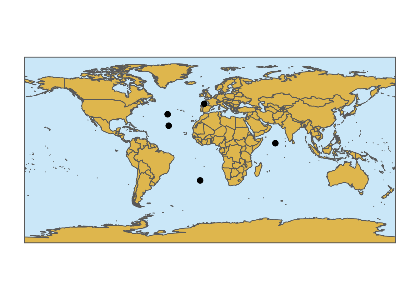
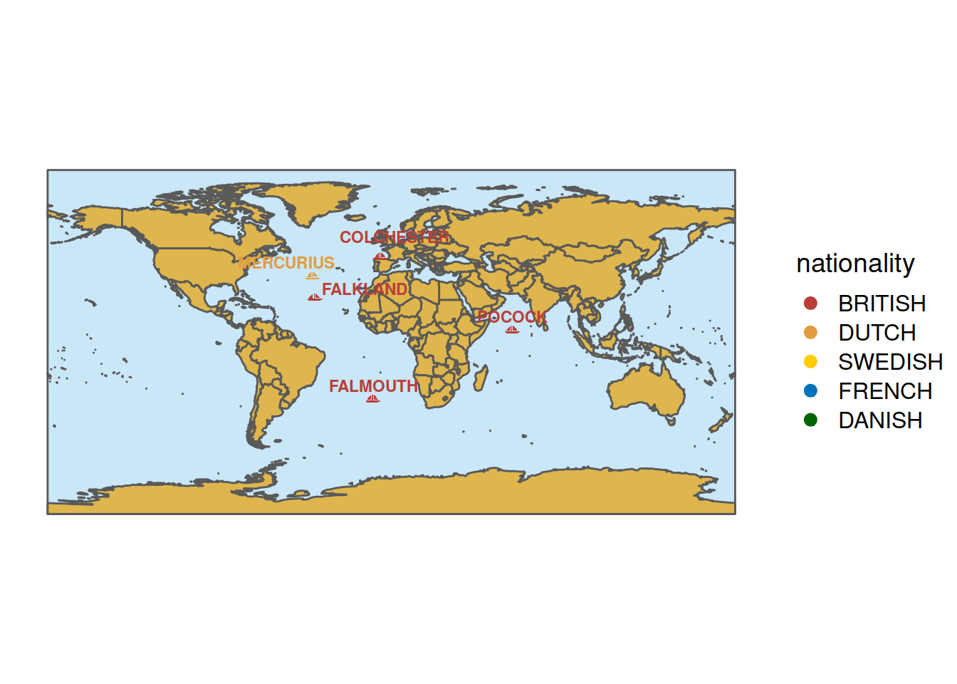
then color by nationality. BUT we want to show all possible values on the legend even though some nationalities aren’t present on this specific day
country_colors <-c("#BA3F38", "#E19C41", "#FFCD00","#0072BB", "darkgreen" )
names(country_colors) <- c("BRITISH","DUTCH", "SWEDISH",  "FRENCH", "DANISH" )

country_colors_scale <-
  scale_colour_manual(
    drop = TRUE,
    limits = names(country_colors), ## les limits (+myColors?) c'est nécessaire pour que toutes les valeurs apparaissent dans la légende même quand pas utilisée.
    values = country_colors)
ggplot() +
geom_sf(data = water_outline, fill = "#56B4E950")+ # blue-coloured water
geom_sf(data = world,
fill = "#E69F00B0") + # brown-coloured background
cowplot::theme_map() +
geom_sf(data = boat_data_1day, aes(color = nationality), size = 3 ) +
country_colors_scale
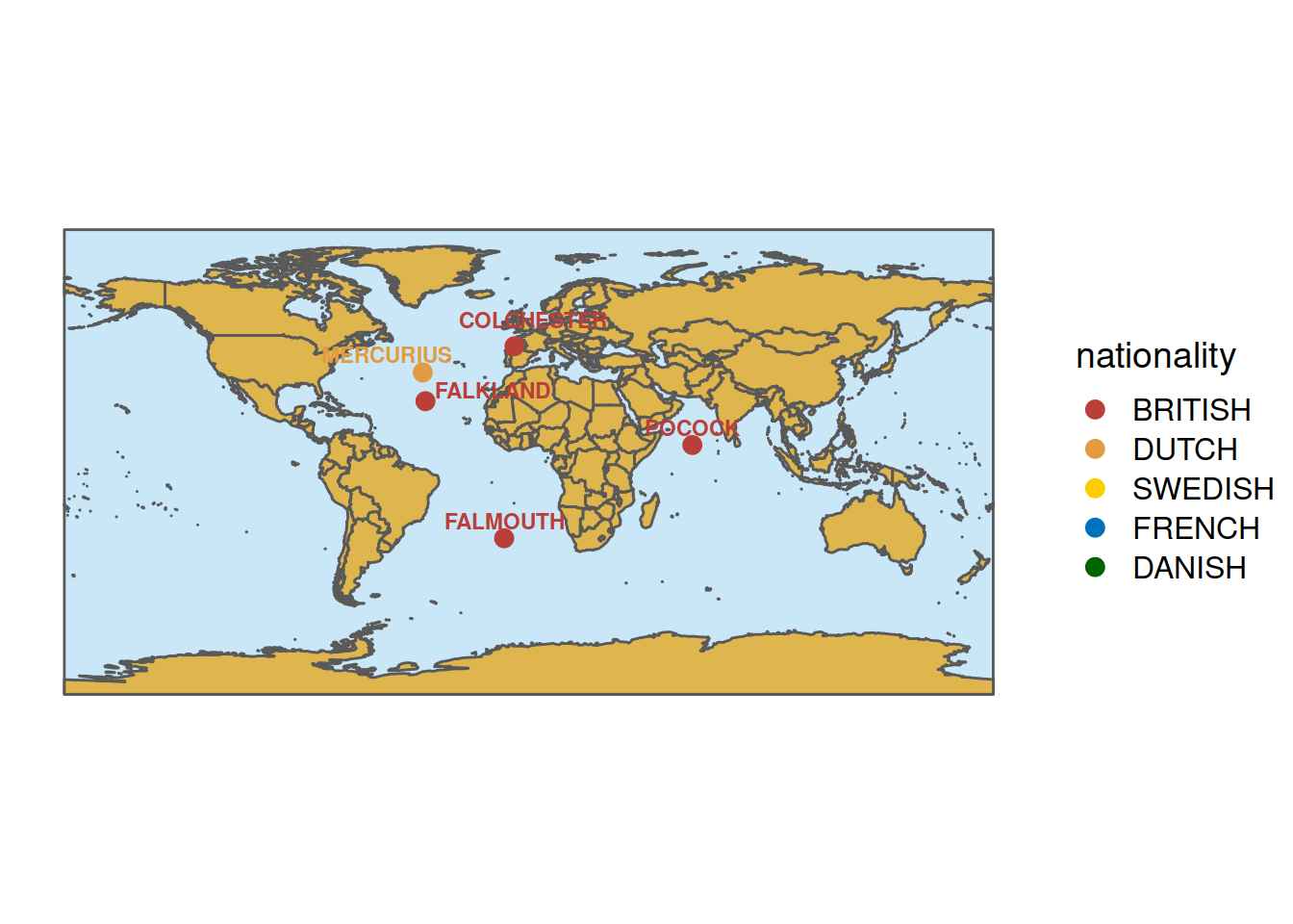
Now let’s add ship names. We have to create a database with columns for the x and y position of the labels, to do this we us st_coordinates() to extract latitude and longitude of the boats.
ggplot() +
  geom_sf(data = water_outline, fill = "#56B4E950")+  # blue-coloured water
  geom_sf(data = world,
          fill = "#E69F00B0")  + # brown-coloured background
  cowplot::theme_map()  +
  geom_sf(data = boat_data_1day, aes(color = nationality), size = 3 ) +
country_colors_scale +
ggrepel::geom_text_repel(
data = boat_data_1day %>%
mutate(
proj_x= map_dbl( geometry, ~st_coordinates(.x)[1]), # trouver les coordonnées projetées
proj_y= map_dbl( geometry, ~st_coordinates(.x)[2])
) %>% st_drop_geometry(), # dropper la géométrie
aes(x = proj_x, y = proj_y, label = ship_name, color = nationality),
fontface = "bold",
size = 3, alpha = 1,
nudge_y = 5 # nudge 2 degrees north
) Next we replace the points with little boat icons. I saved a copy of the icon at “https://blogsimoncoulombe.s3.amazonaws.com/cliwod/sailboat-boat-svgrepo-com.svg”
To do this, we have to use ggimage::geom_image() to display the boats instead of geom_sf()
aws.s3::put_object(file = "/home/simon/git/adhoc_prive/data/downloads/sailboat-boat-svgrepo-com.svg",
                   object = "cliwod/sailboat-boat-svgrepo-com.svg",
                   bucket = "blogsimoncoulombe",
                   acl = "public-read",
                   headers=list("Content-Type" = "image/png")
)
boat_url <- "https://blogsimoncoulombe.s3.amazonaws.com/cliwod/sailboat-boat-svgrepo-com.svg"ggplot() +
geom_sf(data = water_outline, fill = "#56B4E950")+ # blue-coloured water
geom_sf(data = world,
fill = "#E69F00B0") + # brown-coloured background
cowplot::theme_map() +
#geom_sf(data = boat_data_1day, aes(color = nationality), size = 3 ) + ### replaced by boat icons
ggimage::geom_image(data = boat_data_1day %>%
mutate(
proj_x= map_dbl( geometry, ~st_coordinates(.x)[1]), # trouver les coordonnées projetées
proj_y= map_dbl( geometry, ~st_coordinates(.x)[2])
) %>% st_drop_geometry(), # dropper la géométrie
aes(x = proj_x, y = proj_y, color = nationality),
size = 0.02,
image = boat_url
)+
country_colors_scale +
ggrepel::geom_text_repel(
data = boat_data_1day %>%
mutate(
proj_x= map_dbl( geometry, ~st_coordinates(.x)[1]), # trouver les coordonnées projetées
proj_y= map_dbl( geometry, ~st_coordinates(.x)[2])
) %>% st_drop_geometry(), # dropper la géométrie
aes(x = proj_x, y = proj_y, label = ship_name, color = nationality),
fontface = "bold",
size = 3, alpha = 1,
nudge_y = 5 # nudge 2 degrees north
) Add some labels (title, caption) and move the legend on the plot
ggplot() +
geom_sf(data = water_outline, fill = "#56B4E950")+ # blue-coloured water
geom_sf(data = world,
fill = "#E69F00B0") + # brown-coloured background
cowplot::theme_map() +
ggimage::geom_image(data = boat_data_1day %>%
mutate(
proj_x= map_dbl( geometry, ~st_coordinates(.x)[1]), # trouver les coordonnées projetées
proj_y= map_dbl( geometry, ~st_coordinates(.x)[2])
) %>% st_drop_geometry(), # dropper la géométrie
aes(x = proj_x, y = proj_y, color = nationality),
size = 0.02,
image = boat_url
)+
country_colors_scale +
ggrepel::geom_text_repel(
data = boat_data_1day %>%
mutate(
proj_x= map_dbl( geometry, ~st_coordinates(.x)[1]), # trouver les coordonnées projetées
proj_y= map_dbl( geometry, ~st_coordinates(.x)[2])
) %>% st_drop_geometry(), # dropper la géométrie
aes(x = proj_x, y = proj_y, label = ship_name, color = nationality),
fontface = "bold",
size = 3, alpha = 1,
nudge_y = 5 # nudge 2 degrees north
) +
labs(title = "Ship positions on July 1, 1959",
caption = "Gossé par @coulsim \nSource: CLIWOC 2.1",
color = "Nationality") +
theme(legend.position= c(0.05,0.25)) 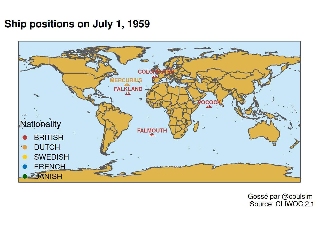 Animate this map over a month using gganimate
plot_july_1959 <- ggplot() +
  geom_sf(data = water_outline, fill = "#56B4E950")+  # blue-coloured water
  geom_sf(data = world,
          fill = "#E69F00B0")  + # brown-coloured background
  cowplot::theme_map()  +
  ggimage::geom_image(data = boat_data_1month %>%
                        mutate(
                          proj_x= map_dbl( geometry, ~st_coordinates(.x)[1]), # trouver les coordonnées projetées
                          proj_y= map_dbl( geometry, ~st_coordinates(.x)[2])
                        ) %>% st_drop_geometry(), # dropper la géométrie
                      aes(x = proj_x, y = proj_y, color = nationality),
                      size = 0.02,
                      image = boat_url
  )+
  country_colors_scale +
  ggrepel::geom_text_repel(
    data = boat_data_1month %>%
      mutate(
        proj_x= map_dbl( geometry, ~st_coordinates(.x)[1]), # trouver les coordonnées projetées
        proj_y= map_dbl( geometry, ~st_coordinates(.x)[2])
      ) %>% st_drop_geometry(), # dropper la géométrie
    aes(x = proj_x, y = proj_y, label = ship_name, color = nationality),
    fontface = "bold",
    size = 3, alpha = 1,
    nudge_y = 5 # nudge 2 degrees north
  ) +
  labs(title =
         "{paste('Ship positions on ',
               lubridate::month(frame_time, label = TRUE, abbr = FALSE),
               lubridate::day(frame_time),
               ',',
               lubridate::year(frame_time)
               )
           }",
       caption = "Gossé par @coulsim \nSource: CLIWOC 2.1",
       color = "Nationality") +
  theme(legend.position= c(0.05,0.25)) +
  transition_time(mydate) +
  ease_aes('linear')

animated_plot_july_1959 <- animate(plot_july_1959, nframes = 36, fps = 10, end_pause = 5, width = 1300, height = 650) # make sure we have at least 1 frame per day.. else we get duplicate ships
anim_save("animated_plot_july_1959.gif", animated_plot_july_1959)

#version mp4 plus petite, mbonne qualité quand même
animated_plot_july_1959_mp4 <- animate(plot1,
                        renderer = ffmpeg_renderer(
                          options = list(vcodec = "libvpx-vp9",
                                         crf = "10",
                                         b = "1600k"
                          )
                        ),
                        nframes = 36,
                        fps = 25, end_pause = 5,
                        width = 1300, height = 650)
anim_save("animated_plot_july_1959.mp4", animated_plot_july_1959_mp4)


aws.s3::put_object(file = "/home/simon/git/snippets/content/post/animated_plot_july_1959.gif",
                   object = "cliwod/animated_plot_july_1959.gif",
                   bucket = "blogsimoncoulombe",
                   acl = "public-read",
                   headers=list("Content-Type" = "image/png")
)

animated_plot_july_1959
Using Winkel-Tripel projection
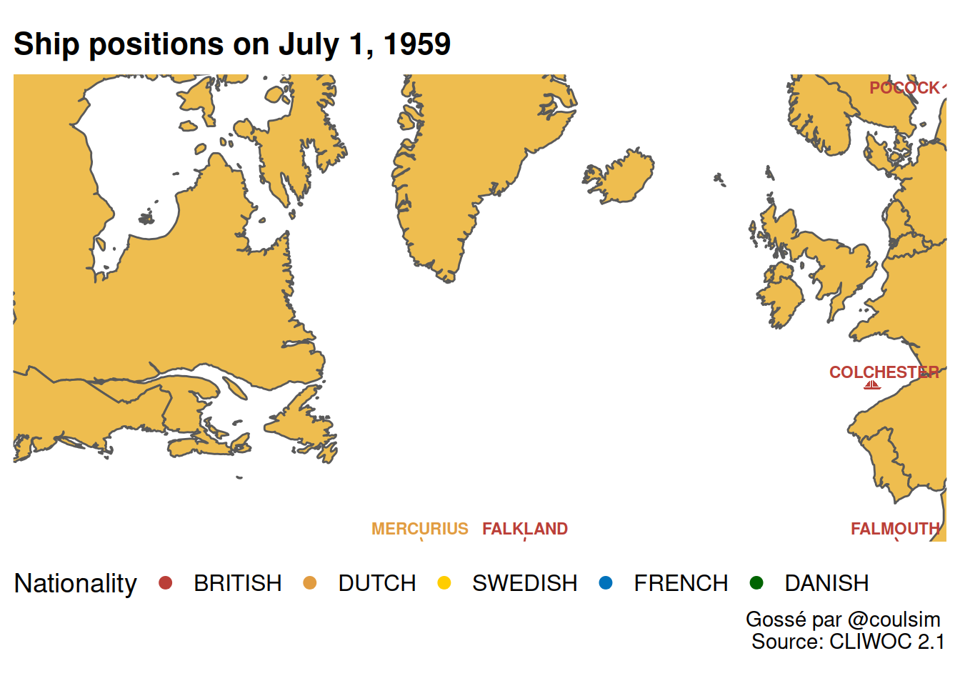
This is NICE!!! .. but what if we’d like to use a projection instead of a rectangle?
I’d like to use winkel-tripel because it’s the projection used by NatGeo.
As far as I know, all we should need to do is
1) reproject all the geom_sf layers (water_outline and world) to winkel-triple using coord_sf("+proj=wintri")
2) manually reproject the labels (in our cases the output of geom_image() and geom_text_repel()) using st_transform(crs= "+proj=wintri") before extracting the coordinates
BUT!!
There is an issue when using Winkel-Tripel with ggplot2. When ggplot2 tries to create a graticule (the grid), it tries to invert the projection and fail (https://github.com/r-spatial/sf/issues/509#issuecomment-340480257).
To get around this, we:
- remove the automatically generated graticule using
coord_sf(datum = NULL) - generate a new graticule using st_graticule() and display it.
This is explaine by Edzer here (https://github.com/r-spatial/sf/issues/509#issuecomment-340492917) and implemented masterfully my Claus Wilke here (https://wilkelab.org/practicalgg/articles/Winkel_tripel.html)
For the water outline, we go back to using geom_sf(data = water_outline) as changing the background added water below Antarctica Also note that the nudge on the ship name has to be increased to a very high number, since the units are different.
ggplot() +
geom_sf(data = water_outline , fill = "#56B4E950")+ # blue-coloured water
geom_sf(data = st_graticule(lat = c(-89.9, seq(-80, 80, 20), 89.9)), color = "gray30", size = 0.25/.pt)+
geom_sf(data = world,
fill = "#E69F00B0") + # brown-coloured background
cowplot::theme_map() +
ggimage::geom_image(data = boat_data_1day %>% st_transform(crs= "+proj=wintri") %>%
mutate(
proj_x= map_dbl( geometry, ~st_coordinates(.x)[1]), # trouver les coordonnées projetées
proj_y= map_dbl( geometry, ~st_coordinates(.x)[2])
) %>% st_drop_geometry(), # dropper la géométrie
aes(x = proj_x, y = proj_y, color = nationality),
size = 0.02,
image = boat_url
)+
country_colors_scale +
ggrepel::geom_text_repel(
data = boat_data_1day %>% st_transform(crs= "+proj=wintri") %>%
mutate(
proj_x= map_dbl( geometry, ~st_coordinates(.x)[1]), # trouver les coordonnées projetées
proj_y= map_dbl( geometry, ~st_coordinates(.x)[2])
) %>% st_drop_geometry(), # dropper la géométrie
aes(x = proj_x, y = proj_y, label = ship_name, color = nationality),
fontface = "bold",
size = 3, alpha = 1,
nudge_y = 500000 # nudge 500000 units north when using winkel-tripel
) +
labs(title = "Winkel-Tripel projection, datum = NULL, manual graticule",
caption = "Gossé par @coulsim \nSource: CLIWOC 2.1",
color = "Nationality") +
theme(legend.position= c(0.03,0.1)) +
coord_sf(
crs = "+proj=wintri" ,
datum = NULL
)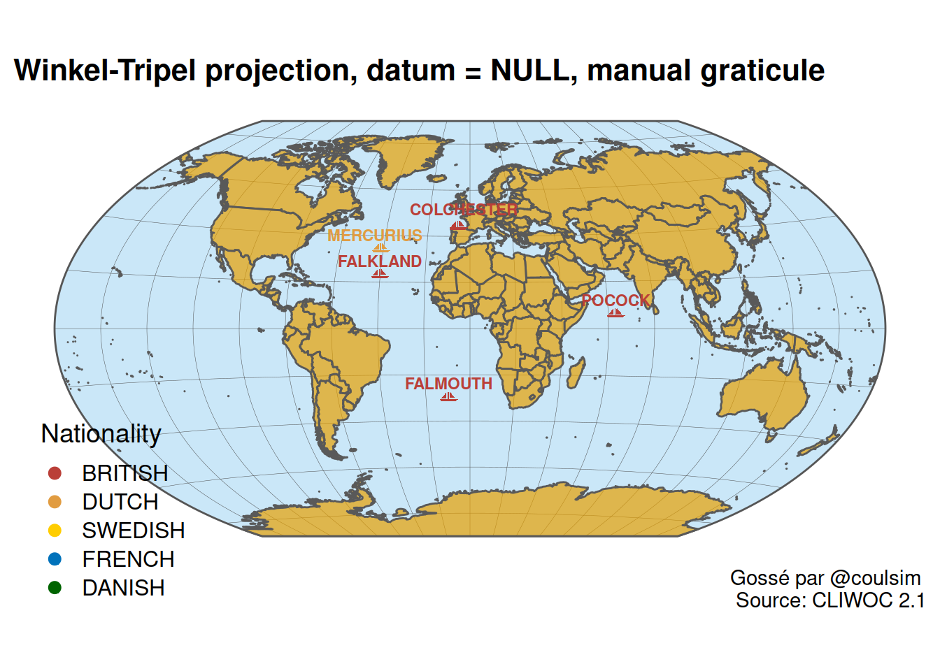 One last thing: I’d like to move the caption and the title on the white space next to the globe.
This is done using negative margins at the bottom for the title and at the top for the caption
theme(plot.title = element_text(margin = margin(b = -60)))
This solution comes from this stackoverflow post : #https://stackoverflow.com/questions/34805506/adjust-title-vertically-to-inside-the-plot-vjust-not-working
ggplot() +
  geom_sf(data = water_outline , fill = "#56B4E950")+  # blue-coloured water
  geom_sf(data = st_graticule(lat = c(-89.9, seq(-80, 80, 20), 89.9)), color = "gray30", size = 0.25/.pt)+
  geom_sf(data = world,
          fill = "#E69F00B0")  + # brown-coloured background
  cowplot::theme_map()  +
  ggimage::geom_image(data = boat_data_1day %>%  st_transform(crs= "+proj=wintri") %>%
                        mutate(
                          proj_x= map_dbl( geometry, ~st_coordinates(.x)[1]), # trouver les coordonnées projetées
                          proj_y= map_dbl( geometry, ~st_coordinates(.x)[2])
                        ) %>% st_drop_geometry(), # dropper la géométrie
                      aes(x = proj_x, y = proj_y, color = nationality),
                      size = 0.02,
                      image = boat_url
  )+
  country_colors_scale +
  ggrepel::geom_text_repel(
    data = boat_data_1day %>%  st_transform(crs= "+proj=wintri") %>%
      mutate(
        proj_x= map_dbl( geometry, ~st_coordinates(.x)[1]), # trouver les coordonnées projetées
        proj_y= map_dbl( geometry, ~st_coordinates(.x)[2])
      ) %>% st_drop_geometry(), # dropper la géométrie
    aes(x = proj_x, y = proj_y, label = ship_name, color = nationality),
    fontface = "bold",
    size = 3, alpha = 1,
    nudge_y = 500000 # nudge 500000 units north when using winkel-tripel
  ) +
  labs(title = "Ship positions on July 1, 1959",
       caption = "Gossé par @coulsim \nSource: CLIWOC 2.1",
       color = "Nationality") +
  theme(legend.position= c(0.03,0.1))  +

  coord_sf(
    crs = "+proj=wintri" ,
    datum  = NULL
  ) +
  theme(plot.title = element_text(margin = margin(b = -60))) +# title inside plot using margin
  theme(plot.caption = element_text(margin = margin(t = -60)))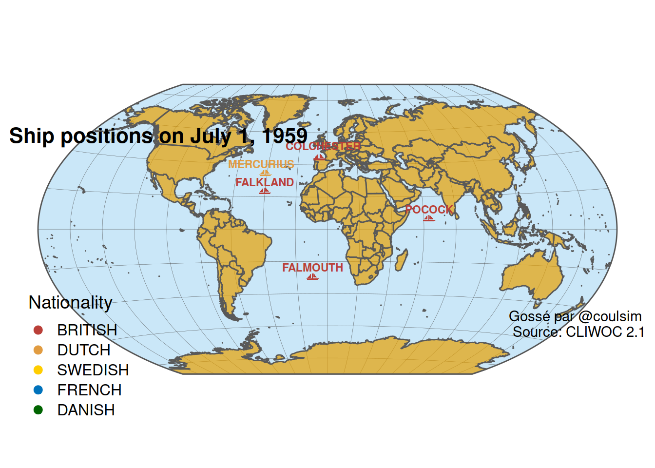
Let’s animate this
animated_plot_july_1959_winkel_tripel <- ggplot() +
  geom_sf(data = water_outline , fill = "#56B4E950")+  # blue-coloured water
  geom_sf(data = st_graticule(lat = c(-89.9, seq(-80, 80, 20), 89.9)), color = "gray30", size = 0.25/.pt)+
  geom_sf(data = world,
          fill = "#E69F00B0")  + # brown-coloured background
  cowplot::theme_map()  +
  ggimage::geom_image(data = boat_data_1month %>%  st_transform(crs= "+proj=wintri") %>%
                        mutate(
                          proj_x= map_dbl( geometry, ~st_coordinates(.x)[1]), # trouver les coordonnées projetées
                          proj_y= map_dbl( geometry, ~st_coordinates(.x)[2])
                        ) %>% st_drop_geometry(), # dropper la géométrie
                      aes(x = proj_x, y = proj_y, color = nationality),
                      size = 0.02,
                      image = boat_url
  )+
  country_colors_scale +
  ggrepel::geom_text_repel(
    data = boat_data_1month %>%  st_transform(crs= "+proj=wintri") %>%
      mutate(
        proj_x= map_dbl( geometry, ~st_coordinates(.x)[1]), # trouver les coordonnées projetées
        proj_y= map_dbl( geometry, ~st_coordinates(.x)[2])
      ) %>% st_drop_geometry(), # dropper la géométrie
    aes(x = proj_x, y = proj_y, label = ship_name, color = nationality),
    fontface = "bold",
    size = 3, alpha = 1,
    nudge_y = 500000 # nudge 500000 units north when using winkel-tripel
  ) +
  labs(title =
         "{paste('Ship positions on ',
               lubridate::month(frame_time, label = TRUE, abbr = FALSE),
               lubridate::day(frame_time),
               ',',
               lubridate::year(frame_time)
               )
           }",
       caption = "Gossé par @coulsim \nSource: CLIWOC 2.1",
       color = "Nationality") +
  theme(legend.position= c(0.03,0.1))  +

  coord_sf(
    crs = "+proj=wintri" ,
    datum  = NULL
  ) +
  theme(plot.title = element_text(margin = margin(b = -60))) +# title inside plot using margin
  theme(plot.caption = element_text(margin = margin(t = -60))) +
  transition_time(mydate) +
  ease_aes('linear')
animated_plot_july_1959_winkel_tripel <- animate(animated_plot_july_1959_winkel_tripel, nframes = 36, fps = 10, end_pause = 5, width = 1300, height = 650) # make sure we have at least 1 frame per day.. else we get duplicate ships
anim_save("animated_plot_july_1959_winkel_tripel.gif", animated_plot_july_1959_winkel_tripel)
aws.s3::put_object(file = "/home/simon/git/snippets/content/post/animated_plot_july_1959_winkel_tripel.gif",
object = "cliwod/animated_plot_july_1959_winkel_tripel.gif",
bucket = "blogsimoncoulombe",
acl = "public-read",
headers=list("Content-Type" = "image/png")
)animated_plot_july_1959_winkel_tripel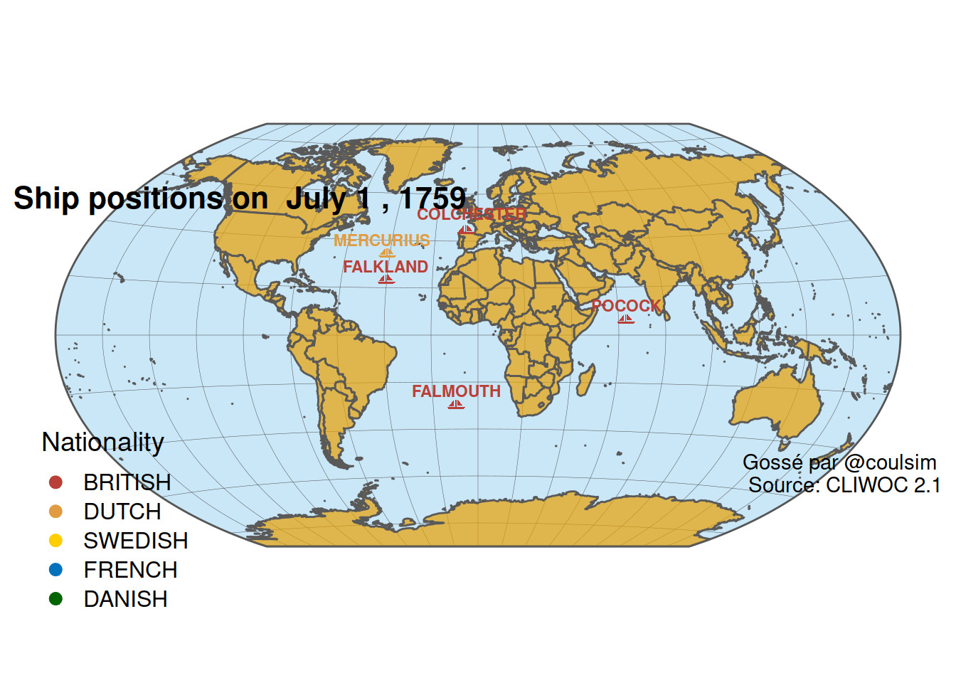

a hope for faster animation : parallel processing using pull request 403 in September 2020
This pull request enables parallel processing: https://github.com/thomasp85/gganimate/issues/78#issuecomment-689855700
devtools::install_github("thomasp85/gganimate", ref = github_pull(403), force= TRUE) After installing, we have to define the number of workers, then run the renderer as usual. I ran into an issue when trying to run on 4 workers
future::plan("multiprocess", workers = 4L)


my_end_pause = 50
my_frames <- as.numeric(max(boat_data_1month$mydate) - min(boat_data_1month$mydate)) + 1 + my_end_pause


animated_mp4 <- animate(animated_plot_july_1959_winkel_tripel,
                        renderer = ffmpeg_renderer(
                          options = list(vcodec = "libvpx-vp9",
                                         crf = "10",
                                         b = "1600k"
                          )
                        ),
                        nframes = my_frames,
                        fps = 25, end_pause = my_end_pause,
                        width = 1300, height = 650)
anim_save("animated_plot_july_1959_winkel_tripel_parallel.mp4", animated_mp4)
[image2 @ 0x5609cbb2e840] Could not open file : /tmp/Rtmph2T1pL/21dc8dee6d6f/gganim_plot0009.png
Input #0, image2, from '/tmp/Rtmph2T1pL/21dc8dee6d6f/gganim_plot%4d.png':
Duration: 00:00:01.20, start: 0.000000, bitrate: N/A
Stream #0:0: Video: png, rgb24(pc), 1300x650, 25 fps, 25 tbr, 25 tbn, 25 tbc
Please use -b:a or -b:v, -b is ambiguous
Stream mapping:
Stream #0:0 -> #0:0 (png (native) -> vp9 (libvpx-vp9))
Press [q] to stop, [?] for help
[image2 @ 0x5609cbb2e840] Could not open file : /tmp/Rtmph2T1pL/21dc8dee6d6f/gganim_plot0009.png
/tmp/Rtmph2T1pL/21dc8dee6d6f/gganim_plot%4d.png: Input/output error
[libvpx-vp9 @ 0x5609cbb37cc0] v1.8.2
Output #0, webm, to '/tmp/Rtmph2T1pL/file21dc843a1ae4f.webm':
Metadata:
encoder : Lavf58.29.100
Stream #0:0: Video: vp9 (libvpx-vp9), gbrp, 1300x650, q=-1--1, 1600 kb/s, 25 fps, 1k tbn, 25 tbc
Metadata:
encoder : Lavc58.54.100 libvpx-vp9
Side data:
cpb: bitrate max/min/avg: 0/0/0 buffer size: 0 vbv_delay: -1
[image2 @ 0x5609cbb2e840] Could not open file : /tmp/Rtmph2T1pL/21dc8dee6d6f/gganim_plot0009.png
/tmp/Rtmph2T1pL/21dc8dee6d6f/gganim_plot%4d.png: Input/output error
[image2 @ 0x5609cbb2e840] Could not open file : /tmp/Rtmph2T1pL/21dc8dee6d6f/gganim_plot0009.png
/tmp/Rtmph2T1pL/21dc8dee6d6f/gganim_plot%4d.png: Input/output error
[image2 @ 0x5609cbb2e840] Could not open file : /tmp/Rtmph2T1pL/21dc8dee6d6f/gganim_plot0009.png
/tmp/Rtmph2T1pL/21dc8dee6d6f/gganim_plot%4d.png: Input/output error
[image2 @ 0x5609cbb2e840] Could not open file : /tmp/Rtmph2T1pL/21dc8dee6d6f/gganim_plot0009.png
/tmp/Rtmph2T1pL/21dc8dee6d6f/gganim_plot%4d.png: Input/output error
[image2 @ 0x5609cbb2e840] Could not open file : /tmp/Rtmph2T1pL/21dc8dee6d6f/gganim_plot0009.png
/tmp/Rtmph2T1pL/21dc8dee6d6f/gganim_plot%4d.png: Input/output error
[image2 @ 0x5609cbb2e840] Could not open file : /tmp/Rtmph2T1pL/21dc8dee6d6f/gganim_plot0009.png
/tmp/Rtmph2T1pL/21dc8dee6d6f/gganim_plot%4d.png: Input/output error
[image2 @ 0x5609cbb2e840] Could not open file : /tmp/Rtmph2T1pL/21dc8dee6d6f/gganim_plot0009.png
/tmp/Rtmph2T1pL/21dc8dee6d6f/gganim_plot%4d.png: Input/output error
frame= 7 fps=0.0 q=0.0 Lsize= 244kB time=00:00:00.24 bitrate=8299.9kbits/s speed=0.245x
video:244kB audio:0kB subtitle:0kB other streams:0kB global headers:0kB muxing overhead: 0.273107%Creating lines (trips) from Points : example using The Hudson Bay Company
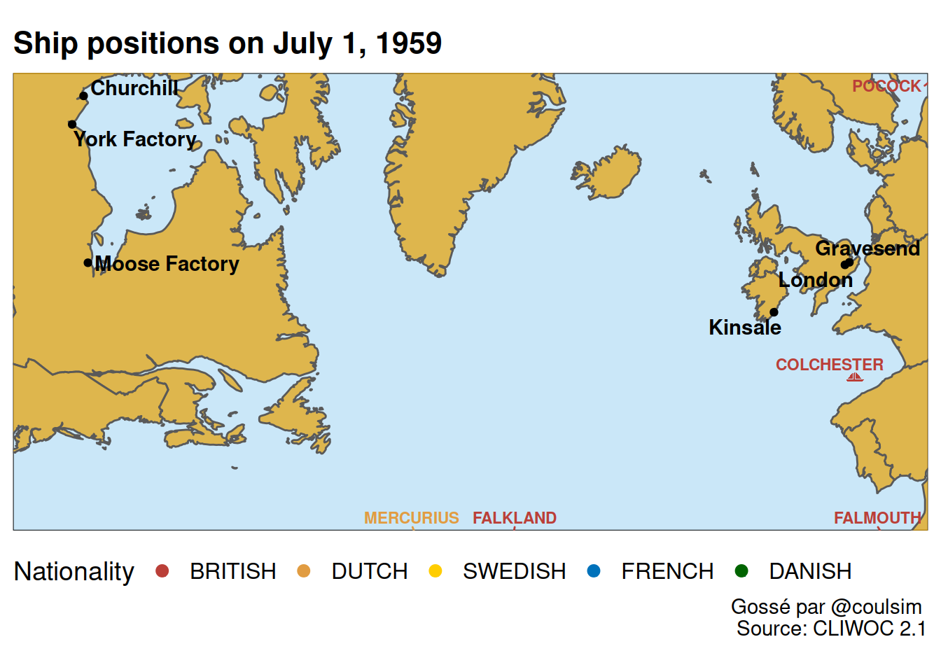
There is one last thing I wanted to do with this dataset. I wanted to show the “lines” of the trips, and I also wanted to zoom into a specific part of the globe.
To do this, we will try to map the trips by the Hudson Bay Company, which are all between England and the Hudson Bay in Canada.
I picked the projection “EPSG: 3574 North Pole LAEA Atlantic”. So we have to do like we did for winkel-tripel: coord_sf( crs = "+init=epsg:3574") for geom_sf() object and st_transform(crs= 3574) for geom_image() and geom_text_repel().
There is an additional difficulty: to zoom into an area, I have to specify coords_sf(xlim = c(), ylim = c()). I found approximage an xlim/ylim window by geocoding two cities I wanted to see on the map (Quebec City and London), then projecting these lat/longs to EPSG 3574 and then adjusting through trial and errors to cover the Hudson Bay.
opencage_forward(placename = "Quebec city") %>%
  .$results %>%
  select(geometry.lat, geometry.lng) %>%
  st_as_sf(coords= c("geometry.lng","geometry.lat"),
           crs = 4326,
           agr = "constant",
           remove = FALSE) %>%
  st_transform(crs = 3574) %>%
  st_coordinates()
## X Y
## 1 -2437821 -4019742opencage_forward(placename = "London, UK") %>%
.$results %>%
head(1) %>%
select(geometry.lat, geometry.lng) %>%
st_as_sf(coords= c("geometry.lng","geometry.lat"),
crs = 4326,
agr = "constant",
remove = FALSE) %>%
st_transform(crs = 3574) %>%
st_coordinates()## X Y
## 1 2701047 -3233585Quebec City is projected to about X = -2.5 million and Y = -4 million. London is projected to about 3 million and -3 million.
My initial window was xlim = c(-3e6, 3e6) and ylim = c(-5e6, -3e6), but trial and error showed that I needed to add space to the West to reach the Hudson Bay and North to include Greenland, so I ended up with the following limits:
coord_sf(
  crs = "+init=epsg:3574",
  xlim = c(-5e6,  5e6), ylim = c(-5e6, -1e6)
)
Transformed coordinates used by geom_image() and geom_text_repel() to EPSG 3574 by using the st_transform() function. The result is below:
ggplot() +
  geom_sf(data = water_outline , fill = "#56B4E950")+  # blue-coloured water
  geom_sf(data = world,
          fill = "#E69F00B0")  + # brown-coloured background
  cowplot::theme_map()  +
  ggimage::geom_image(data = boat_data_1day %>%  st_transform(crs= 3574) %>%
                        mutate(
                          proj_x= map_dbl( geometry, ~st_coordinates(.x)[1]), # trouver les coordonnées projetées
                          proj_y= map_dbl( geometry, ~st_coordinates(.x)[2])
                        ) %>% st_drop_geometry(), # dropper la géométrie
                      aes(x = proj_x, y = proj_y, color = nationality),
                      size = 0.02,
                      image = boat_url
  )+
  country_colors_scale +
  ggrepel::geom_text_repel(
    data = boat_data_1day %>%  st_transform(crs= 3574) %>%
      mutate(
        proj_x= map_dbl( geometry, ~st_coordinates(.x)[1]), # trouver les coordonnées projetées
        proj_y= map_dbl( geometry, ~st_coordinates(.x)[2])
      ) %>% st_drop_geometry(), # dropper la géométrie
    aes(x = proj_x, y = proj_y, label = ship_name, color = nationality),
    fontface = "bold",
    size = 3, alpha = 1,
    nudge_y = 5 # nudge 2 degrees north
  ) +
  labs(title = "Ship positions on July 1, 1959",
       caption = "Gossé par @coulsim \nSource: CLIWOC 2.1",
       color = "Nationality") +
  theme(legend.position= "bottom") +
  coord_sf(
    crs = "+init=epsg:3574",
    xlim = c(-3e6,  3e6), ylim = c(-5e6, -2e6)
  )
This isnt too bad, but my water outline is gone.
The easiest workaround I found is to change the plot background to blue using theme(panel.background = element_rect(fill = "#56B4E950")).
ggplot() +
  #geom_sf(data = water_outline , fill = "#56B4E950")+  # blue-coloured water
  geom_sf(data = world,
          fill = "#E69F00B0")  + # brown-coloured background
  cowplot::theme_map()  +
  ggimage::geom_image(data = boat_data_1day %>%  st_transform(crs= 3574) %>%
                        mutate(
                          proj_x= map_dbl( geometry, ~st_coordinates(.x)[1]), # trouver les coordonnées projetées
                          proj_y= map_dbl( geometry, ~st_coordinates(.x)[2])
                        ) %>% st_drop_geometry(), # dropper la géométrie
                      aes(x = proj_x, y = proj_y, color = nationality),
                      size = 0.02,
                      image = boat_url
  )+
  country_colors_scale +
  ggrepel::geom_text_repel(
    data = boat_data_1day %>%  st_transform(crs= 3574) %>%
      mutate(
        proj_x= map_dbl( geometry, ~st_coordinates(.x)[1]), # trouver les coordonnées projetées
        proj_y= map_dbl( geometry, ~st_coordinates(.x)[2])
      ) %>% st_drop_geometry(), # dropper la géométrie
    aes(x = proj_x, y = proj_y, label = ship_name, color = nationality),
    fontface = "bold",
    size = 3, alpha = 1,
    nudge_y = 5 # nudge 2 degrees north
  ) +
  labs(title = "Ship positions on July 1, 1959",
       caption = "Gossé par @coulsim \nSource: CLIWOC 2.1",
       color = "Nationality") +
  theme(legend.position= "bottom") +
  coord_sf(
    crs = "+init=epsg:3574",
    xlim = c(-3e6,  3e6), ylim = c(-5e6, -2e6)
  )+
  theme(panel.background = element_rect(fill = "#56B4E950"))
Let’s add points of interests to the map.
We just geocode 6 cities using
Let’s add points of interests to the map.
We just geocode 6 cities using opencageand project them using st_transform() then add them using geom_text_repel() and geom_point()
moose_factory <- opencage_forward(placename = "Moose Factory, Ontario") %>%
  .$results %>% head(1) %>%
  select(geometry.lat, geometry.lng) %>%
  mutate(nom = "Moose Factory")


york_factory <- opencage_forward(placename = "York Factory, Manitoba") %>%
  .$results %>% head(1) %>%
  select(geometry.lat, geometry.lng) %>%
  mutate(nom = "York Factory")


churchill <- opencage_forward(placename = "Churchill, Manitoba") %>%
  .$results %>% head(1) %>%
  select(geometry.lat, geometry.lng) %>%
  mutate(nom = "Churchill")

gravesend <- opencage_forward(placename = "GRAVESEND, ENGLAND") %>%
  .$results %>% head(1) %>%
  select(geometry.lat, geometry.lng) %>%
  mutate(nom = "Gravesend")

kinsale <- opencage_forward(placename = "KINSALE, IRELAND") %>%
  .$results %>% head(1) %>%
  select(geometry.lat, geometry.lng) %>%
  mutate(nom = "Kinsale")

london <- opencage_forward(placename = "LONDON, ENGLAND") %>%
  .$results %>% head(1) %>%
  select(geometry.lat, geometry.lng) %>%
  mutate(nom = "London")


villes <- bind_rows(
  moose_factory, york_factory, churchill, kinsale, gravesend, london
) %>%
  st_as_sf(coords= c("geometry.lng","geometry.lat"),
           crs = 4326,
           agr = "constant",
           remove = FALSE)
ggplot() +
#geom_sf(data = water_outline , fill = "#56B4E950")+ # blue-coloured water
geom_sf(data = world,
fill = "#E69F00B0") + # brown-coloured background
cowplot::theme_map() +
ggimage::geom_image(data = boat_data_1day %>% st_transform(crs= 3574) %>%
mutate(
proj_x= map_dbl( geometry, ~st_coordinates(.x)[1]), # trouver les coordonnées projetées
proj_y= map_dbl( geometry, ~st_coordinates(.x)[2])
) %>% st_drop_geometry(), # dropper la géométrie
aes(x = proj_x, y = proj_y, color = nationality),
size = 0.02,
image = boat_url
)+
country_colors_scale +
ggrepel::geom_text_repel(
data = boat_data_1day %>% st_transform(crs= 3574) %>%
mutate(
proj_x= map_dbl( geometry, ~st_coordinates(.x)[1]), # trouver les coordonnées projetées
proj_y= map_dbl( geometry, ~st_coordinates(.x)[2])
) %>% st_drop_geometry(), # dropper la géométrie
aes(x = proj_x, y = proj_y, label = ship_name, color = nationality),
fontface = "bold",
size = 3, alpha = 1,
nudge_y = 5 # nudge 2 degrees north
) +
labs(title = "Ship positions on July 1, 1959",
caption = "Gossé par @coulsim \nSource: CLIWOC 2.1",
color = "Nationality") +
theme(legend.position= "bottom") +
coord_sf(
crs = "+init=epsg:3574",
xlim = c(-3e6, 3e6), ylim = c(-5e6, -2e6)
)+
theme(panel.background = element_rect(fill = "#56B4E950")) +
geom_point(data = villes %>%
st_transform(crs= 3574) %>% # projeter les villes
mutate(
lon= map_dbl( geometry, ~st_coordinates(.x)[1]), # trouver les coordonnées projetées
lat= map_dbl( geometry, ~st_coordinates(.x)[2])
) %>% st_drop_geometry(), # dropper la géométrie
aes(x = lon, y = lat)
) +
ggrepel::geom_text_repel(data = villes %>%
st_transform(crs= 3574) %>% # projeter les villes
mutate(
lon= map_dbl( geometry, ~st_coordinates(.x)[1]), # trouver les coordonnées projetées
lat= map_dbl( geometry, ~st_coordinates(.x)[2])
) %>% st_drop_geometry(), # dropper la géométrie
aes(x = lon, y = lat, label = nom), #
fontface = "bold"
) 
Finally, we create lines to represent all the trips made by the Hudson Bay Company back over that period.
trips_hudson_bay_company <- mycliwoc  %>%
  filter(company == "HUDSON BAY COMPANY")  %>%
  group_by(ship_name, voyage_ini, voyage_ini_year)%>%
  arrange(mydate) %>%
  summarize(., do_union = FALSE) %>%
  st_cast("LINESTRING")
ggplot() +
geom_sf(data = world,
fill = "#E69F00B0") + # brown-coloured background
cowplot::theme_map() +
geom_sf(data =trips_hudson_bay_company,
aes(color = as.factor(voyage_ini_year)),
alpha =0.7)+
labs(
title = "Voyages de 4 bateaux de la Compagnie de la Baie d'Hudson (1760-1799)",
subtitle = "On nomme les postes de traite 'factory' (manufactures), car en anglais le nom d’un commerçant est dit 'factor'",
caption = "Source: CLIWOC 2.1 (https://www.historicalclimatology.com/uploads/4/5/1/4/4514421/cliwoc21.ods) \n
gossé par @coulsim, couleurs de @ClausWilke, projection: EPSG: 3574 North Pole LAEA Atlantic",
color = "Année"
) +
coord_sf(
crs = "+init=epsg:3574",
xlim = c(-3e6, 3e6), ylim = c(-5e6, -1e6)
)+
theme(panel.background = element_rect(fill = "#56B4E950")) +
geom_point(data = villes %>%
st_transform(crs= 3574) %>% # projeter les villes
mutate(
lon= map_dbl( geometry, ~st_coordinates(.x)[1]), # trouver les coordonnées projetées
lat= map_dbl( geometry, ~st_coordinates(.x)[2])
) %>% st_drop_geometry(), # dropper la géométrie
aes(x = lon, y = lat)
) +
ggrepel::geom_text_repel(data = villes %>%
st_transform(crs= 3574) %>% # projeter les villes
mutate(
lon= map_dbl( geometry, ~st_coordinates(.x)[1]), # trouver les coordonnées projetées
lat= map_dbl( geometry, ~st_coordinates(.x)[2])
) %>% st_drop_geometry(), # dropper la géométrie
aes(x = lon, y = lat, label = nom), #
fontface = "bold"
) +
facet_wrap(~ ship_name)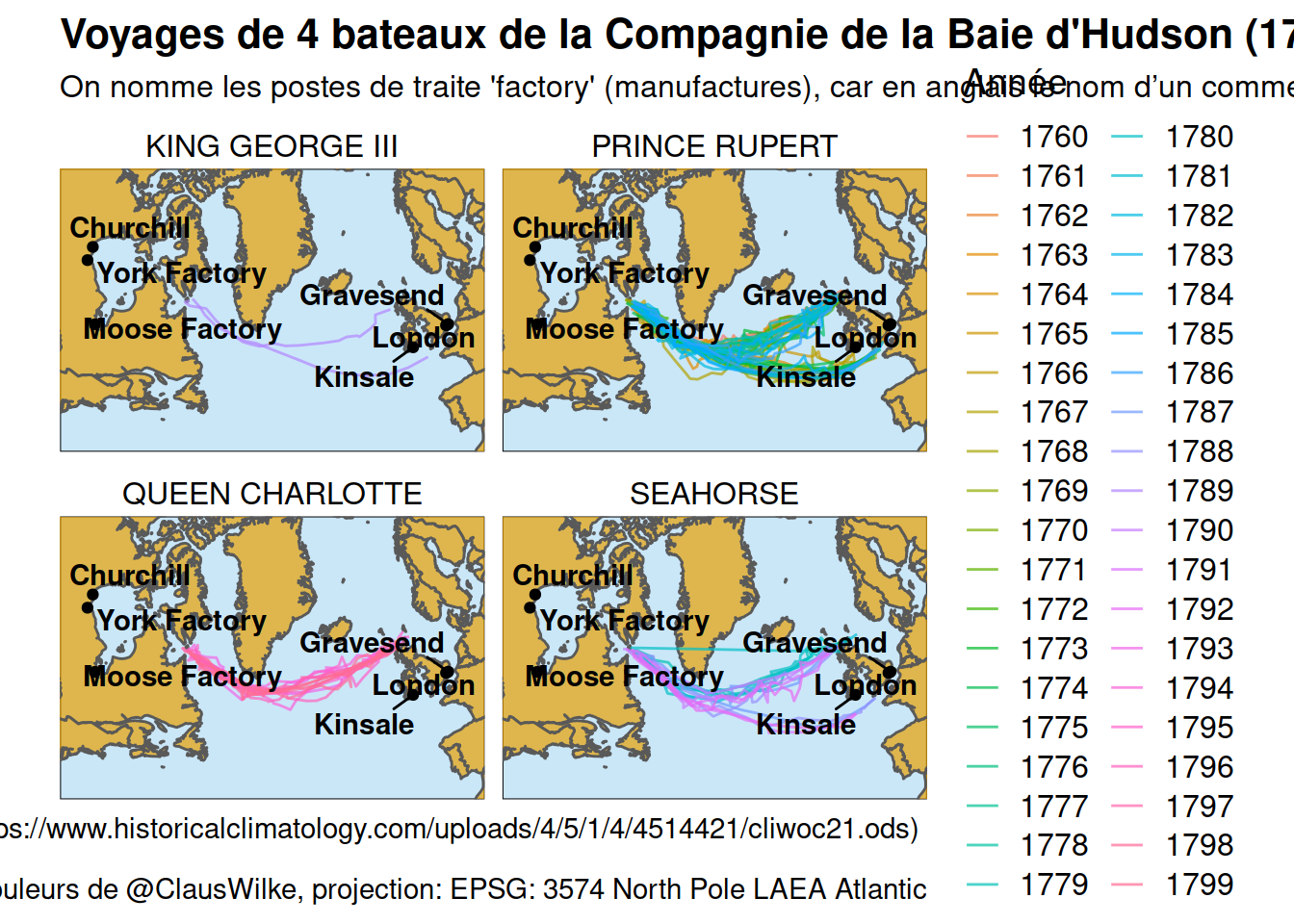
that’s it folks!