
tidymodels and insurance loss cost models
- Objective
- The data
- {rsample} Grouped and stratified train/test split and resamples
- {doMC} Set up parallel processing
- Logistic Regression with formula pre-processor
- Logistic Regression with recipe pre-processor
- Tweedie regression
- TODO: Poisson regression
- TODO: Gamma regression
- resources
Objective
I want to implement a tweedie regression similar to what one would face in the insurance industry using the {tidymodels} ecosystem.
Some context: I built my first tweedie regression model three years ago. That blog post was also the first time I used the recipes and rsample packages and I have been a huge fan since then. However, I delayed trying parsnip and workflows packages until today because I felt that many of the specifics of my models were hard to implement using these packages.
Here’s a list of “new to me” stuff I do in the code below that work:
- use
rsamplefunctionsgroup_initial_split()andgroup_vfold_cv()to do a “grouped” train/test data split. This is often required when using insurance data because a givenpolicy_idwill have multiple rows and I want all rows for a given policy to be either in train or test rather than spread all over the place,
- use case weights (in my case,
exposure),
- use
embed::step_lencode_glm()to replace high-cardinality variables with embedded values,
- use
GLM,GAM,xgboostandlightgbmmodel specifications and check that the output is the same as fitting the models outside of tidymodels. Spoiler : for GAMs you need to pass a formula with theadd_model()or theupdate_workflow_model()functions,
- create
tweedieregressions and check that the output is the same as what I would get by fitting the models outside of tidymodels .
- use workflow sets to apply the same pre-processors (recipe or formula) to a bunch of model specifications and pick the best one using cross validation. bonus: tune some hyperparameters at the same time.
Things I would like to figure out eventually:
- is weighted normalized gini available? Useful when evaluating tweedie regression. (order by predicted annual loss, but weight with exposure). As used in the “fire peril loss cost kaggle” (https://www.kaggle.com/c/liberty-mutual-fire-peril/discussion/9880) or seen in this yardstick issue (https://github.com/tidymodels/yardstick/issues/442).
- figure out a way to use GAMs with splines when using a recipe pre-processor (how can I craft a formula when I dont know the variable names created by the recipe step_dummy and step_other functions and these variables could change for each resample?,
- how to weight records using
exposurewhen creating the train/test split and the resamples so that all resamples have the same total exposure rather than the same number of records,
- figure out a way to use case weights in
lightgbm,
- create
poissonandgammaregressions (should be similar to tweedie, but I’m out of time).
Let’s get started!
The data
Copying from my 2020 post, here is the description of the data:
The dataCar data from the insuranceData package. It contains 67 856 one-year vehicle insurance policies taken out in 2004 or 2005. It originally came with the book Generalized Linear Models for Insurance Data (2008).
The presence of a claim is indicated by the clm (0 or 1) , which indicates that there is at least one claim. We will rename the variable to has_claim.
The total dollar value of claims for a given period is claimcst0, which we will rename to dollar_loss. We will divide it by the exposure to obtain loss_cost, the dollar loss per year.
The exposure variable represents the “number of years of exposure” and is used as the case weight variable. It is bound between 0 and 1.
The independent variables are as follow:
veh_value, the vehicle value in tens of thousand of dollars,
veh_body, vehicle body, coded as 13 different values: BUS CONVT COUPE HBACK HDTOP MCARA MIBUS PANVN RDSTR SEDAN STNWG TRUCK UTE,
veh_age, 1 (youngest), 2, 3, 4,
gender, a factor with levels F M,
areaa factor with levels A B C D E F,
agecat1 (youngest), 2, 3, 4, 5, 6
The loss_cost variable is what actuaries want to model (and charge you with a slight markup). In insurance, it is typically modelled directly using a tweedieregression, or indirectly by multiplying the output of two models, one predicting the frequency of claims (poisson regression) and the other predicting the severity of claims (gamma regression).
NOTE: While the end goal of this blog post is to model the loss_cost, I will start with baby steps and start with modelling has_claim_fct using logistic regression.
Note: when using the frequency*severity approach, we will use the has_claim_fct variable in the Poisson (frequency) variable instead of numclaims (actual number of claims) because we don’t have the breakdown of the value of each claims when there is more than one. In practice, this means modelling “a lower frequency multiplied with an higher average severity” than reality, but the overall predicted annual loss will be the same.
I create exposure_weight, which is the result of hardhat::importance_weights(exposure). This will often allow us to pass weights to the tidymodels use_case_weights() function.
I also create a factor has_claim_fct because parsnip want classification models to work on factors, not integers.
FUN #1: I am going to create a fake policy_id column, which has a 10% chance of being the same as the row above it. This is to represent that a policy_id can have multiple records. I will want all records for a given policy to be in the same resample.
set.seed(42)

data(dataCar)

# claimcst0 = claim amount in dollars (0 if no claim)
# clm = 0 or 1 = has a claim yes/ no
#  numclaims = number of claims  0 , 1 ,2 ,3 or 4).
# we use clm because the corresponding dollar amount is for all claims combined.
mydb <- dataCar %>%
  select(has_claim = clm, dollar_loss= claimcst0, exposure, veh_value, veh_body,
         veh_age, gender, area, agecat) %>%
  mutate(
    loss_cost = dollar_loss / exposure,
    policy_id =1,
    random = runif(nrow(.)),
    has_claim_fct = factor(if_else(has_claim==1, "yes", "no"), levels = c("yes", "no")),
    exposure_weight = hardhat::importance_weights(exposure)
  )


# ugly and slow, but this is what I could come up with quickly
for (i in seq(from =2, to =nrow(mydb))){
  if (mydb[i,"random"]< 0.2 ){
    mydb[i,"policy_id"] <-  mydb[i-1,"policy_id"]
  } else{
    mydb[i,"policy_id"] <-  mydb[i-1,"policy_id"] +1
  }
}

mydb %>%
  count(policy_id) %>%
  count(n) %>%
  gt(caption="most (fake) policy_id have only 1 record in the dataset, but many have more",
  ) %>%
cols_width( everything() ~ px(200))| n | nn |
|---|---|
| 1 | 43148 |
| 2 | 8660 |
| 3 | 1790 |
| 4 | 380 |
| 5 | 79 |
| 6 | 16 |
| 7 | 1 |
{rsample} Grouped and stratified train/test split and resamples
We want all the records for a given policy_id to end up in either train or test. We also want to try to have roughly the same annual loss in the train and test.
To do this, we use recipes::group_initial_split() to group by policy_id and stratify by loss_cost.
set.seed(123)
try(my_split <- group_initial_split( mydb, group = policy_id, prop= 3/4, strata = loss_cost))
## Error in check_grouped_strata({ :
## `strata` must be constant across all members of each `group`.oooh ! our first error.: “strata must be constant across all members of each group.”. This happens because some records for a given policy will have a claim and other won’t. I’m going to calculate an average loss_cost over all records for a given policy_id. I would love to be able to weight records by exposure (to have the same total exposure and average loss_cost in all resamples), but I don’t think that’s possible.
here we go:
mydb <- mydb %>%
  group_by(policy_id) %>%
  mutate(policy_loss_cost = sum( dollar_loss) / sum(exposure)) %>%
  ungroup()

set.seed(123)
my_split <- group_initial_split( mydb, group = policy_id, prop= 3/4, strata = policy_loss_cost) # this works!

my_train <- training(my_split)
my_test  <- testing(my_split)
are any policy_id split between train and test? No. (this is what we wanted)
both <- bind_rows(
  my_train %>% mutate(type = "train"),
  my_test %>% mutate(type = "test"),
)


both %>%
  distinct(policy_id, type) %>%
  count(policy_id) %>%
  count(n) %>%
  gt(caption = "all policy_id are seen in only 1 type (either train or test), never both") %>%
cols_width( everything() ~ px(200))| n | nn |
|---|---|
| 1 | 54074 |
Is the proportion of records 3/4 train and 1/4 test? Yes!
both %>%
  count(type) %>%
  mutate(pct = n/sum(n)) %>%
  gt(caption="proportion of records in train/test is exactly  75% vs 25%, as expected") %>%
cols_width( everything() ~ px(200))| type | n | pct |
|---|---|---|
| test | 16963 | 0.2499853 |
| train | 50893 | 0.7500147 |
however, exposure isnt spread 75%/25%. This is normal because we couldnt weight records in the group_initial_split() function, but this would have been nice:
both %>%
  group_by(type) %>%
  summarise(exposure = sum(exposure)) %>%
  mutate(pct = exposure/sum(exposure)) %>%
  gt(caption="exposure is NOT split exactly  75-25 because we couldnt weight records when splitting") %>%
cols_width( everything() ~ px(200))| type | exposure | pct |
|---|---|---|
| test | 7961.977 | 0.2503702 |
| train | 23838.842 | 0.7496298 |
We tried to stratify our groups using the policy_loss_cost variable. However, some policies have more exposure than other. This means that the average annual loss for the train/test won’t be identical. How different are they? It appears we got lucky and outliers didnt mess too much with our averages:
both %>%
  group_by(type) %>%
  summarise(overall_loss_cost = sum(dollar_loss)/ sum(exposure)) %>%
  ungroup() %>%
  gt(caption="overall annuall loss (dollar loss per year ) isnt the same in both train and test") %>%
cols_width( everything() ~ px(200))The overall frequency should also be different between train and test. It shouldnt be as volatile because frequency depends only on frequency (duh), while annual loss depends on frequency and severity.
both %>%
  group_by(type) %>%
  summarise(overall_frequency = sum(has_claim)/ sum(exposure)) %>%
  ungroup() %>%
  gt(caption="overall frequency (claims per year) is less different  between train and test  than the overall annual loss") %>%
cols_width( everything() ~ px(200))| type | overall_frequency |
|---|---|
| test | 0.1451901 |
| train | 0.1454769 |
to create folds , we use the group_vfold_cv, again stratified over policy_loss_cost
set.seed(234)
train_resamples <- group_vfold_cv(my_train,
                                  group="policy_id",
                                  strata = policy_loss_cost,
                                  v= 5)
I won’t check the overall annual loss and overall frequency for each resamples, but the volatility here would be interesting to look at.
{doMC} Set up parallel processing
We are going to run a lot of models when fitting models on multiples resamples and multiple hyperparameter sets. tune_grid() can use multiple cores if we tell it to:
doMC::registerDoMC(cores = 6)Logistic Regression with formula pre-processor
We need to learn to walk before we learn to run. So I’m going to try building a logistic regression before diving into the “complicated” models like tweedie, poisson and gamma.
Let’s just pretend everyone has the same exposure and create a simple logistic regression on whether or not a record has a claim.
Here’s the formula for my logistic regression:
my_logistic_reg_formula <- as.formula("has_claim_fct ~ veh_value + veh_body + veh_age + gender + area + agecat")Reproducing “non-tidymodels” specs in tidymodels
Before diving into the cool stuff like evaluating the model on multiple resamples and tuning parameters, I’ll just make sure I can reproduce the model fit inside and outside tidymodels
GLM (unweighted)
The code below to generate the specification for a GLM logistic regression was initially generated by running parsnip::parsnip_addin(), selecting classification, logistic_reg (glm) and unchecking tag parameters for tuning (if any) then clicking the gren write specification code button.
Tidymodels output
logistic_glm_spec <-
  parsnip::logistic_reg() %>%
  parsnip::set_engine("glm")

logistic_glm_fit <-logistic_glm_spec %>%
  parsnip::fit(
    formula = my_logistic_reg_formula,
    data = my_train)

logistic_glm_fit %>%
  extract_fit_engine() %>%
  tidy()
## # A tibble: 22 × 5
## term estimate std.error statistic p.value
## <chr> <dbl> <dbl> <dbl> <dbl>
## 1 (Intercept) 1.20 0.443 2.71 0.00670
## 2 veh_value -0.0543 0.0207 -2.62 0.00879
## 3 veh_bodyCONVT 2.25 0.849 2.65 0.00796
## 4 veh_bodyCOUPE 0.963 0.453 2.12 0.0337
## 5 veh_bodyHBACK 1.28 0.431 2.97 0.00300
## 6 veh_bodyHDTOP 1.12 0.442 2.54 0.0111
## 7 veh_bodyMCARA 0.532 0.530 1.00 0.316
## 8 veh_bodyMIBUS 1.44 0.466 3.09 0.00198
## 9 veh_bodyPANVN 1.05 0.455 2.30 0.0216
## 10 veh_bodyRDSTR 1.25 0.856 1.46 0.144
## # ℹ 12 more rowsNon-tidymodels output
is this the same output as directly running the normal glm?
yes!
glm(my_logistic_reg_formula,    family = "binomial", data = my_train)  %>%
  tidy()
## # A tibble: 22 × 5
## term estimate std.error statistic p.value
## <chr> <dbl> <dbl> <dbl> <dbl>
## 1 (Intercept) 1.20 0.443 2.71 0.00670
## 2 veh_value -0.0543 0.0207 -2.62 0.00879
## 3 veh_bodyCONVT 2.25 0.849 2.65 0.00796
## 4 veh_bodyCOUPE 0.963 0.453 2.12 0.0337
## 5 veh_bodyHBACK 1.28 0.431 2.97 0.00300
## 6 veh_bodyHDTOP 1.12 0.442 2.54 0.0111
## 7 veh_bodyMCARA 0.532 0.530 1.00 0.316
## 8 veh_bodyMIBUS 1.44 0.466 3.09 0.00198
## 9 veh_bodyPANVN 1.05 0.455 2.30 0.0216
## 10 veh_bodyRDSTR 1.25 0.856 1.46 0.144
## # ℹ 12 more rowsGLM (weighted)
What if we want to weights records? It doesnt really make sense in this logistic example, but will in the future for the loss_cost model. . Apparently we can use add_case_weights() and refer to the exposure_weight column of type importance_weight we created earlier:
Tidymodels output
weighted_logistic_glm_wf <-   workflow() %>%
  add_case_weights(exposure_weight) %>%
  add_formula(my_logistic_reg_formula) %>%
  add_model(logistic_glm_spec)

weighted_logistic_glm_wf_fit <-  weighted_logistic_glm_wf%>%
  fit(data = my_train)

weighted_logistic_glm_wf_fit %>% tidy()
## # A tibble: 22 × 5
## term estimate std.error statistic p.value
## <chr> <dbl> <dbl> <dbl> <dbl>
## 1 (Intercept) 0.634 0.544 1.17 0.243
## 2 veh_value -0.0461 0.0271 -1.70 0.0893
## 3 veh_bodyCONVT 1.99 1.03 1.93 0.0539
## 4 veh_bodyCOUPE 1.03 0.563 1.83 0.0667
## 5 veh_bodyHBACK 1.41 0.527 2.68 0.00729
## 6 veh_bodyHDTOP 1.20 0.541 2.22 0.0262
## 7 veh_bodyMCARA 0.625 0.676 0.923 0.356
## 8 veh_bodyMIBUS 1.42 0.574 2.46 0.0137
## 9 veh_bodyPANVN 1.13 0.556 2.04 0.0417
## 10 veh_bodyRDSTR 0.934 1.02 0.916 0.360
## # ℹ 12 more rowsNon-tidymodels output
is it the same a directly modelling outside tidymodels? Yes!
glm(my_logistic_reg_formula, family = "binomial", data = my_train, weights = exposure) %>% tidy()## # A tibble: 22 × 5
## term estimate std.error statistic p.value
## <chr> <dbl> <dbl> <dbl> <dbl>
## 1 (Intercept) 0.634 0.544 1.17 0.243
## 2 veh_value -0.0461 0.0271 -1.70 0.0893
## 3 veh_bodyCONVT 1.99 1.03 1.93 0.0539
## 4 veh_bodyCOUPE 1.03 0.563 1.83 0.0667
## 5 veh_bodyHBACK 1.41 0.527 2.68 0.00729
## 6 veh_bodyHDTOP 1.20 0.541 2.22 0.0262
## 7 veh_bodyMCARA 0.625 0.676 0.923 0.356
## 8 veh_bodyMIBUS 1.42 0.574 2.46 0.0137
## 9 veh_bodyPANVN 1.13 0.556 2.04 0.0417
## 10 veh_bodyRDSTR 0.934 1.02 0.916 0.360
## # ℹ 12 more rowsGAM (with splines) (weighted)
- Note 1: the REML method is passed to set_engine() rather than gen_additive_mod() because this option is specific to the mgcv package.
- Note 2: GAMs need us to specify the formula twice, once in add_model() and another time in add_formula. Interesting: I need to add the spline in the formula in add_model(my_logistic_reg_formula_with_splines), but not in add_formula(my_logistic_reg_formula). more here : https://community.rstudio.com/t/how-to-define-smoothed-models-for-a-gam-using-tidymodels-and-recipe/144772/2
- Note 3: I need to add
parametric=TRUEto broom::tidy() to get the mgcv parameters (https://broom.tidymodels.org/reference/tidy.gam.html). Te default (parametric=FALSE) returns the fitted spline.
# parsnip_addin()

logistic_gam_spec <-
  gen_additive_mod() %>%
  set_engine('mgcv', method= "REML") %>%
  set_mode('classification')

my_logistic_reg_formula_with_splines <- as.formula('has_claim_fct ~ s(veh_value, bs= "tp") + veh_body + veh_age +  gender +  area +  agecat')


logistic_gam_wf <- workflow() %>%
  add_model(logistic_gam_spec, formula = my_logistic_reg_formula_with_splines) %>%  # need to add formula twice, and  in add_formula
  add_formula(my_logistic_reg_formula) %>%
  add_case_weights(exposure_weight)


logistic_gam_wf_fit <-  logistic_gam_wf%>%
  fit(data = my_train )


logistic_gam_wf_fit %>% tidy(parametric = TRUE)
## # A tibble: 21 × 5
## term estimate std.error statistic p.value
## <chr> <dbl> <dbl> <dbl> <dbl>
## 1 (Intercept) 0.789 0.542 1.45 0.146
## 2 veh_bodyCONVT 1.66 1.04 1.60 0.110
## 3 veh_bodyCOUPE 0.982 0.566 1.74 0.0826
## 4 veh_bodyHBACK 1.32 0.531 2.48 0.0131
## 5 veh_bodyHDTOP 1.27 0.545 2.34 0.0195
## 6 veh_bodyMCARA 0.709 0.679 1.04 0.296
## 7 veh_bodyMIBUS 1.50 0.578 2.60 0.00945
## 8 veh_bodyPANVN 1.11 0.559 1.98 0.0475
## 9 veh_bodyRDSTR 0.872 1.02 0.853 0.394
## 10 veh_bodySEDAN 1.30 0.530 2.46 0.0138
## # ℹ 11 more rowssame result if I do it directly using mgcv::gam? Yes!
mgcv::gam(
  formula = my_logistic_reg_formula_with_splines,
  data = my_train,
  weights = exposure,
  family = stats::binomial(link = "logit"),
  method="REML") %>%
  broom::tidy(parametric= TRUE)
## # A tibble: 21 × 5
## term estimate std.error statistic p.value
## <chr> <dbl> <dbl> <dbl> <dbl>
## 1 (Intercept) 0.789 0.542 1.45 0.146
## 2 veh_bodyCONVT 1.66 1.04 1.60 0.110
## 3 veh_bodyCOUPE 0.982 0.566 1.74 0.0826
## 4 veh_bodyHBACK 1.32 0.531 2.48 0.0131
## 5 veh_bodyHDTOP 1.27 0.545 2.34 0.0195
## 6 veh_bodyMCARA 0.709 0.679 1.04 0.296
## 7 veh_bodyMIBUS 1.50 0.578 2.60 0.00945
## 8 veh_bodyPANVN 1.11 0.559 1.98 0.0475
## 9 veh_bodyRDSTR 0.872 1.02 0.853 0.394
## 10 veh_bodySEDAN 1.30 0.530 2.46 0.0138
## # ℹ 11 more rowsXGBoost (weighted)
Let’s start with specifying all the hyperparameters manually. Tuning will have to wait for now.
logistic_xgb_spec <-
  boost_tree(
    tree_depth = 3,
    trees= 200,
    learn_rate = 0.1,
    min_n = 50,
    loss_reduction = 0,
    sample_size = 1.0,
    stop_iter = 50
  ) %>%
  set_engine('xgboost', nthread = 1) %>%
  set_mode('classification')

logistic_xgb_wf <- workflow() %>%
  add_model(logistic_xgb_spec) %>%
  add_formula(my_logistic_reg_formula) %>%
  add_case_weights(exposure_weight)

set.seed(345)
logistic_xgb_wf_fit <-  logistic_xgb_wf%>%
  fit(data = my_train )


logistic_xgb_wf_fit %>% extract_fit_engine() %>% vip::vip(num_features= 30L)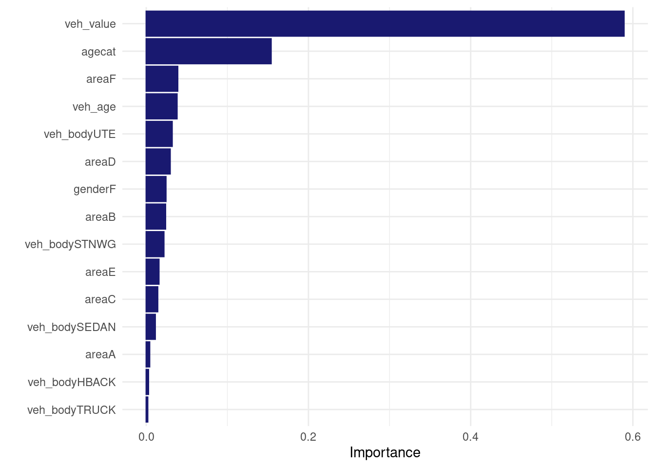
Can I train the exact same thing using xgboost directly?
Answer: YES!
NOTE: I need to one-hot encode dummy variables to match what {tidymodels} do.
my_recipe <- recipe(my_train ) %>%
update_role(all_of(labels(terms(my_logistic_reg_formula))), new_role = "predictor") %>%
update_role(has_claim, new_role= "outcome") %>%
update_role(exposure, new_role = "weight") %>%
step_dummy(all_nominal_predictors(), one_hot = TRUE) %>% ## APPARENTLY tidymodels use one_hot = TRUE because their model has 24 features. when I dont set one_hot I only have 21 features.
step_select(has_role(c("predictor", "outcome", "weight")))
prepped_recipe <- prep(my_recipe)
baked_train <- bake(prepped_recipe, my_train)
baked_test <- bake(prepped_recipe, my_test)
my_params <- list(
eta = 0.1,
max_depth = 3,
gamma = 0,
colsample_bytree = 1,
colsample_bynode = 1,
min_child_weight = 50,
subsample = 1,
nthread = 1)
xgtrain <- xgboost::xgb.DMatrix(
data = as.matrix(baked_train %>% select(-has_claim, -exposure)),
label = baked_train$has_claim,
weight = baked_train$exposure
)
xgtest <- xgboost::xgb.DMatrix(
data = as.matrix(baked_test %>% select(-has_claim, -exposure)),
label = baked_test$has_claim,
weight = baked_test$exposure
)
set.seed(345)
direct_xgb_fit <- xgboost::xgb.train(
data = xgtrain,
params = my_params,
nrounds = 200,
objective = "binary:logistic"
)
vip::vip(direct_xgb_fit, num_features = 30L)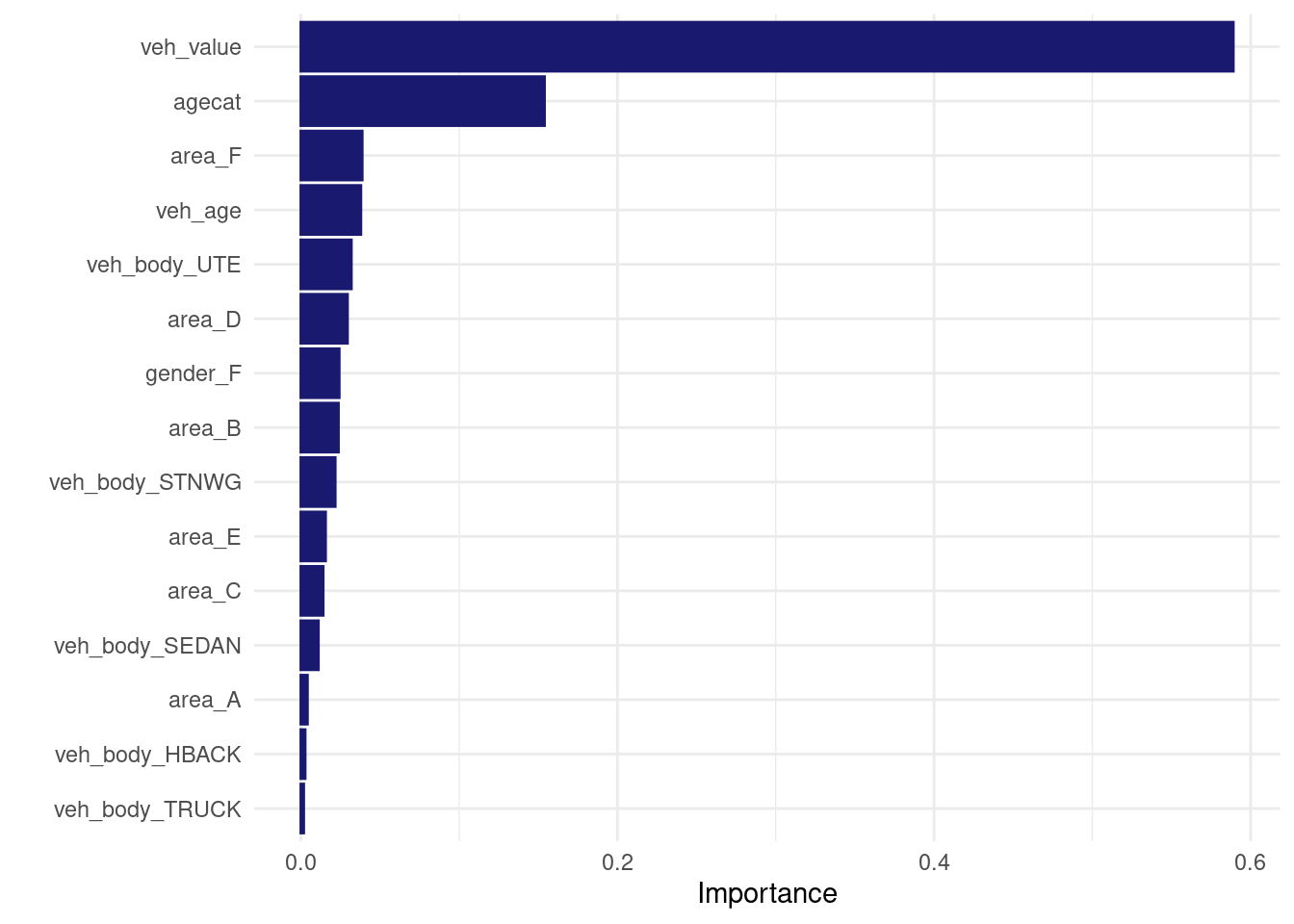 Same predictions for the first.. 6 digits?
pred_tidy <- predict(logistic_xgb_wf_fit, new_data = my_test, type = "prob")   %>% select(.pred_yes)
pred_direct <- predict(direct_xgb_fit, newdata = xgtest)
z <- pred_tidy %>% rename(pred_tidy = .pred_yes) %>%  add_column(pred_direct)
z %>% ggplot(aes(x= pred_tidy, y = pred_direct)) +
  geom_point(alpha = 0.05) +
  geom_smooth() +
  coord_equal()
Identical first tree:
tidymodels xgboost model tree #1:
xgb.plot.tree(model = logistic_xgb_wf_fit %>% extract_fit_engine(), trees = 1)direct xgboost model tree #1:
xgb.plot.tree(model = direct_xgb_fit, trees = 1)same parameters:
tidymodels parameters:
logistic_xgb_wf_fit %>% extract_fit_engine()## ##### xgb.Booster
## raw: 202.8 Kb
## call:
## xgboost::xgb.train(params = list(eta = 0.1, max_depth = 3, gamma = 0,
## colsample_bytree = 1, colsample_bynode = 1, min_child_weight = 50,
## subsample = 1), data = x$data, nrounds = 200, watchlist = x$watchlist,
## verbose = 0, early_stopping_rounds = 50, nthread = 1, objective = "binary:logistic")
## params (as set within xgb.train):
## eta = "0.1", max_depth = "3", gamma = "0", colsample_bytree = "1", colsample_bynode = "1", min_child_weight = "50", subsample = "1", nthread = "1", objective = "binary:logistic", validate_parameters = "TRUE"
## xgb.attributes:
## best_iteration, best_msg, best_ntreelimit, best_score, niter
## callbacks:
## cb.evaluation.log()
## cb.early.stop(stopping_rounds = early_stopping_rounds, maximize = maximize,
## verbose = verbose)
## # of features: 24
## niter: 200
## best_iteration : 200
## best_ntreelimit : 200
## best_score : 0.2954026
## best_msg : [200] training-logloss:0.295403
## nfeatures : 24
## evaluation_log:
## iter training_logloss
## 1 0.6288661
## 2 0.5763974
## ---
## 199 0.2954106
## 200 0.2954026direct fit parameters:
direct_xgb_fit## ##### xgb.Booster
## raw: 202.6 Kb
## call:
## xgboost::xgb.train(params = my_params, data = xgtrain, nrounds = 200,
## objective = "binary:logistic")
## params (as set within xgb.train):
## eta = "0.1", max_depth = "3", gamma = "0", colsample_bytree = "1", colsample_bynode = "1", min_child_weight = "50", subsample = "1", nthread = "1", objective = "binary:logistic", validate_parameters = "TRUE"
## xgb.attributes:
## niter
## callbacks:
## cb.print.evaluation(period = print_every_n)
## # of features: 24
## niter: 200
## nfeatures : 24looks likes I managed to get the same thing
lightgbm (unweighted)
Here’s how to create a lightgbm model in tidymodels. TODO :try to reproduce it by fitting it directly (outside tidymodels)
logistic_lightgbm_spec <-
  boost_tree(
    trees= 200
  ) %>%
  set_engine('lightgbm') %>%  # num_leaves = tune()
  set_mode('classification')

logistic_lightgbm_wf <- workflow() %>%
  add_model(logistic_lightgbm_spec) %>%
  add_formula(my_logistic_reg_formula)


set.seed(345)
logistic_lightgbm_wf_fit <-  logistic_lightgbm_wf%>%
  fit(data = my_train ) # Case weights are not enabled by the underlying model implementation.


logistic_lightgbm_wf_fit %>% extract_fit_engine() %>% vip::vip()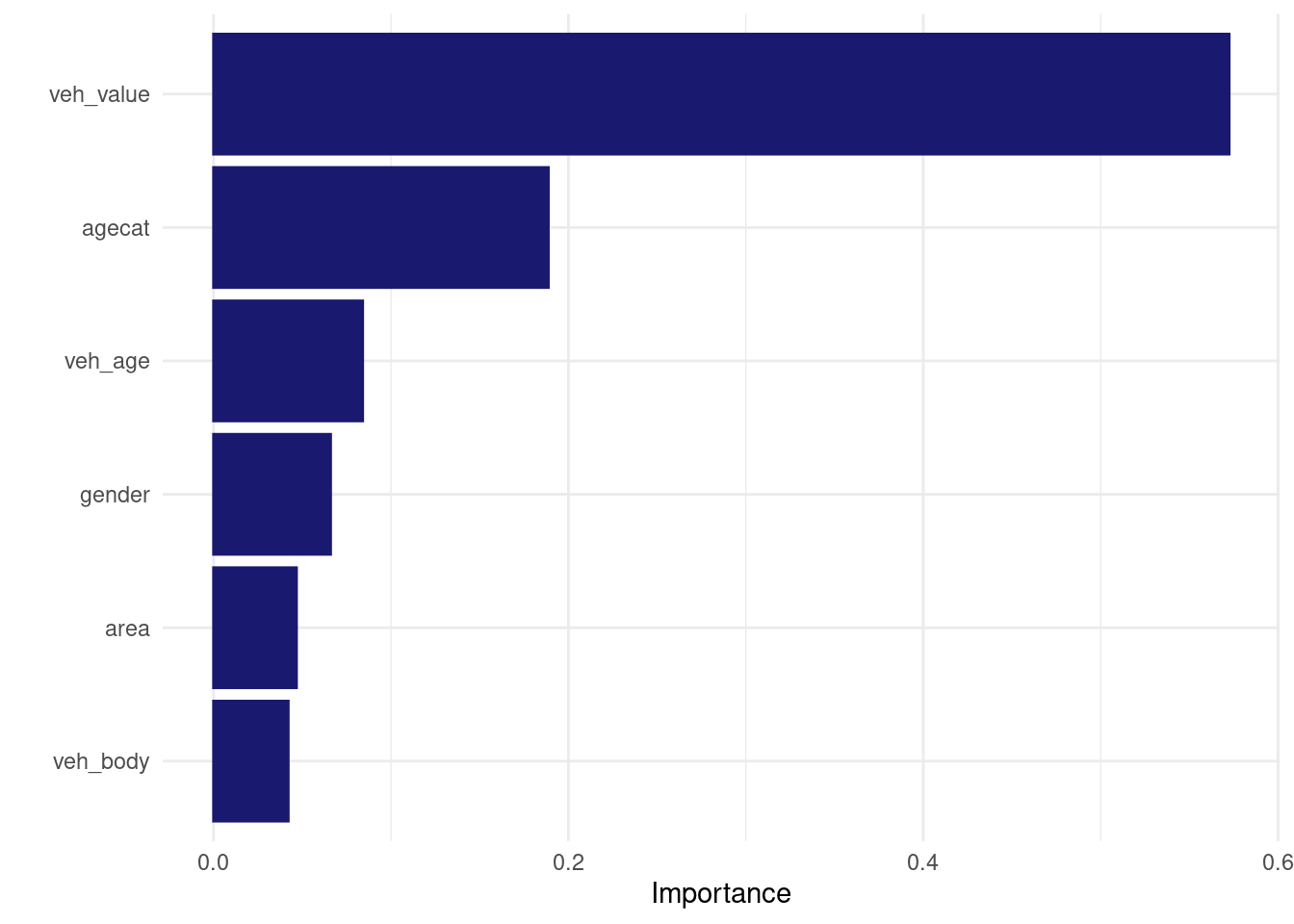
lightgbm weighted (not implemented in tidymodels)
appears not possible at the moment:
TL;DR: Case weights are not enabled by the underlying model implementation.
try(
  workflow() %>%
    add_model(logistic_lightgbm_spec) %>%
    add_formula(my_logistic_reg_formula)  %>%
    add_case_weights(exposure_weight) %>%
    fit(data = my_train )
)
## Error in check_case_weights(case_weights, object) :
## Case weights are not enabled by the underlying model implementation.Use workflow_set to fit all logitics models specification on all resamples
Alright, that was fun! Now that I feel I know how to train a model in tidymodels, let’s try to define all the models at once using a preprocessor and a list of model specifications. Then we apply fit_resamples() to fit all workflows to all resamples.
In our case, the pre-processor is a formula, but we could have used a recipe as the preprocessor. We’ll try that in another part later (named “Logistic Regression with recipe pre-processor”).
This workflow_set will be mapped to the fit_resamples() to fit all models on all folds. Tuning will be in another part using the tune_grid function.
NOTE 1 : update_workflow_model() exists https://github.com/tidymodels/workflowsets/issues/64 and is used to add the formula to the GAM model inside a workflow_set.
NOTE 2 : we’re could have used a list multiple different pre-processors to test different model specifications. we’ll try that in a part later.
all_workflows <-
  workflow_set(
    preproc = list("formula"= my_logistic_reg_formula ),
    models = list(
      logistic_glm = logistic_glm_spec,
      logistic_gam = logistic_gam_spec,
      logistic_xgboost = logistic_xgb_spec
    ),
    case_weights = exposure_weight
  )

all_workflows <- update_workflow_model(all_workflows,
                                       i =  "formula_logistic_gam",
                                       spec = logistic_gam_spec,
                                       formula = my_logistic_reg_formula)

# Workflows can take special arguments for the recipe (e.g. a blueprint) or a model (e.g. a special formula). However, when creating a workflow set, there is no way to specify these extra components. update_workflow_model() and update_workflow_recipe() allow users to set these values after the workflow set is initially created. They are analogous to workflows::add_model() or workflows::add_recipe().

all_workflows2 <-
  all_workflows %>%
  workflow_map(resamples = train_resamples,
               fn = "fit_resamples",
               verbose = TRUE)
rank_results(all_workflows2, rank_metric = "roc_auc")## # A tibble: 6 × 9
## wflow_id .config .metric mean std_err n preprocessor model rank
## <chr> <chr> <chr> <dbl> <dbl> <int> <chr> <chr> <int>
## 1 formula_logistic… Prepro… accura… 0.932 0.00133 5 formula logi… 1
## 2 formula_logistic… Prepro… roc_auc 0.540 0.00112 5 formula logi… 1
## 3 formula_logistic… Prepro… accura… 0.932 0.00133 5 formula gen_… 2
## 4 formula_logistic… Prepro… roc_auc 0.540 0.00112 5 formula gen_… 2
## 5 formula_logistic… Prepro… accura… 0.932 0.00133 5 formula boos… 3
## 6 formula_logistic… Prepro… roc_auc 0.539 0.00273 5 formula boos… 3autoplot(all_workflows2, metric="roc_auc")
Add hyperparameter tuning to the workflow_set
ok, that was fun. Here’s how to do try with a grid of hyperparameters
logistic_tuneable_xgb_spec <-
  boost_tree(
    trees= 200,
    learn_rate = 0.05,
    tree_depth = tune(),
    min_n = tune(),
    loss_reduction = 0,
    sample_size = 1,
    mtry= 1, # colsample_bynode
    stop_iter = 50
  ) %>%
  set_engine('xgboost', nthread = 1) %>%
  set_mode('classification')
create a grid with 12 different sets of hyperparameters.
set.seed(789)
my_grid <- grid_latin_hypercube(
  tree_depth(range = c(2,10)),
  min_n(),
  size = 12
)
all_workflows3 <-
workflow_set(
preproc = list("formula"= my_logistic_reg_formula ),
models = list(
logistic_glm = logistic_glm_spec,
logistic_gam = logistic_gam_spec,
logistic_xgboost = logistic_xgb_spec,
logistic_tuneable_xgb = logistic_tuneable_xgb_spec
),
case_weights = exposure_weight
)
all_workflows3 <- update_workflow_model(all_workflows3,
i = "formula_logistic_gam",
spec = logistic_gam_spec,
formula = my_logistic_reg_formula)
# Workflows can take special arguments for the recipe (e.g. a blueprint) or a model (e.g. a special formula). However, when creating a workflow set, there is no way to specify these extra components. update_workflow_model() and update_workflow_recipe() allow users to set these values after the workflow set is initially created. They are analogous to workflows::add_model() or workflows::add_recipe().
all_workflows4 <-
all_workflows3 %>%
#option_add(control = control_grid(save_pred = TRUE), grid = 12) %>%
option_add(control = control_grid(save_pred = TRUE), grid = my_grid) %>%
workflow_map(resamples = train_resamples,
fn = "tune_grid",
verbose = TRUE,
seed = 567) this time we have a lot more of boosted trees because logistic_tuneable_xgb goes through a grid of 12 sets of hyperparameters. (most of which are shitty..)
autoplot(all_workflows4, metric="roc_auc")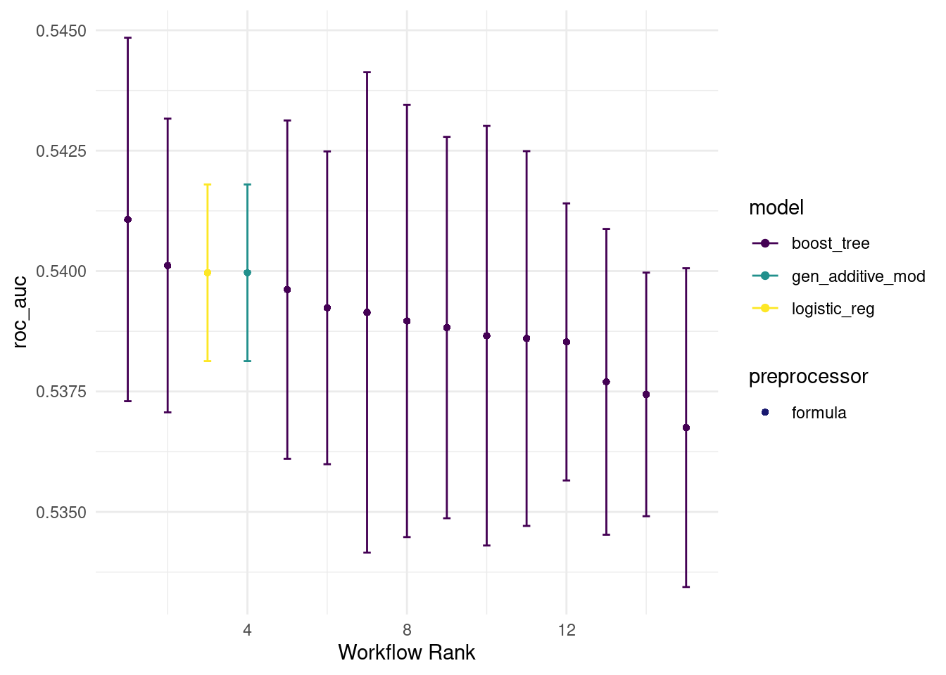
rank_results(all_workflows4, rank_metric = "roc_auc") %>% filter(.metric == "roc_auc")## # A tibble: 15 × 9
## wflow_id .config .metric mean std_err n preprocessor model rank
## <chr> <chr> <chr> <dbl> <dbl> <int> <chr> <chr> <int>
## 1 formula_logisti… Prepro… roc_auc 0.541 0.00229 5 formula boos… 1
## 2 formula_logisti… Prepro… roc_auc 0.540 0.00185 5 formula boos… 2
## 3 formula_logisti… Prepro… roc_auc 0.540 0.00112 5 formula logi… 3
## 4 formula_logisti… Prepro… roc_auc 0.540 0.00112 5 formula gen_… 4
## 5 formula_logisti… Prepro… roc_auc 0.540 0.00213 5 formula boos… 5
## 6 formula_logisti… Prepro… roc_auc 0.539 0.00197 5 formula boos… 6
## 7 formula_logisti… Prepro… roc_auc 0.539 0.00303 5 formula boos… 7
## 8 formula_logisti… Prepro… roc_auc 0.539 0.00273 5 formula boos… 8
## 9 formula_logisti… Prepro… roc_auc 0.539 0.00241 5 formula boos… 9
## 10 formula_logisti… Prepro… roc_auc 0.539 0.00265 5 formula boos… 10
## 11 formula_logisti… Prepro… roc_auc 0.539 0.00237 5 formula boos… 11
## 12 formula_logisti… Prepro… roc_auc 0.539 0.00175 5 formula boos… 12
## 13 formula_logisti… Prepro… roc_auc 0.538 0.00193 5 formula boos… 13
## 14 formula_logisti… Prepro… roc_auc 0.537 0.00154 5 formula boos… 14
## 15 formula_logisti… Prepro… roc_auc 0.537 0.00201 5 formula boos… 15note: we can compare the out-of-sample predictions of all models using collect_predictions(all_workflows4). Here are the predictions of all 15 models for the first row in test:
out_of_sample_preds <- collect_predictions(all_workflows4)
out_of_sample_preds %>% filter(.row ==1) %>% arrange(desc(.pred_yes))
## # A tibble: 15 × 9
## wflow_id .config preproc model .row has_claim_fct .pred_yes .pred_no
## <chr> <chr> <chr> <chr> <int> <fct> <dbl> <dbl>
## 1 formula_logisti… Prepro… formula boos… 1 no 0.0846 0.915
## 2 formula_logisti… Prepro… formula boos… 1 no 0.0843 0.916
## 3 formula_logisti… Prepro… formula boos… 1 no 0.0842 0.916
## 4 formula_logisti… Prepro… formula boos… 1 no 0.0841 0.916
## 5 formula_logisti… Prepro… formula boos… 1 no 0.0814 0.919
## 6 formula_logisti… Prepro… formula boos… 1 no 0.0813 0.919
## 7 formula_logisti… Prepro… formula boos… 1 no 0.0813 0.919
## 8 formula_logisti… Prepro… formula logi… 1 no 0.0811 0.919
## 9 formula_logisti… Prepro… formula gen_… 1 no 0.0811 0.919
## 10 formula_logisti… Prepro… formula boos… 1 no 0.0808 0.919
## 11 formula_logisti… Prepro… formula boos… 1 no 0.0802 0.920
## 12 formula_logisti… Prepro… formula boos… 1 no 0.0801 0.920
## 13 formula_logisti… Prepro… formula boos… 1 no 0.0800 0.920
## 14 formula_logisti… Prepro… formula boos… 1 no 0.0787 0.921
## 15 formula_logisti… Prepro… formula boos… 1 no 0.0744 0.926
## # ℹ 1 more variable: .pred_class <fct>just making sure.. is my weighted average pred equal to my weighted average “has_claim” for my logistic_glm workflow? yup
my_train %>% add_column(
  out_of_sample_preds %>%
    filter(wflow_id=="formula_logistic_glm") %>%
    select(.pred_yes)
) %>%
  summarise(weighted_average_pred = sum(exposure * .pred_yes)/sum(exposure),
            weighted_average_has_claim = sum(has_claim * exposure) / sum(exposure)
  )
## # A tibble: 1 × 2
## weighted_average_pred weighted_average_has_claim
## <dbl> <dbl>
## 1 0.0888 0.0889Here the best modelon set of hyperparameters from “formula_logistic_tuneable_xgb” workflow. Let’s extract that workflow, then show the best 5 results and finally select_best() hyperparameters and finalise the logistic_tuneable_xgb by running the model on the whole training set with the best hyperparameters.
logistic_tuneable_xgb_wf_result <-
  all_workflows4 %>%
  extract_workflow_set_result("formula_logistic_tuneable_xgb")

logistic_tuneable_xgb_wf_result %>% show_best(metric = "roc_auc")
## # A tibble: 5 × 8
## min_n tree_depth .metric .estimator mean n std_err .config
## <int> <int> <chr> <chr> <dbl> <int> <dbl> <chr>
## 1 12 9 roc_auc binary 0.541 5 0.00229 Preprocessor1_Model01
## 2 8 6 roc_auc binary 0.540 5 0.00185 Preprocessor1_Model11
## 3 15 10 roc_auc binary 0.540 5 0.00213 Preprocessor1_Model04
## 4 35 9 roc_auc binary 0.539 5 0.00197 Preprocessor1_Model02
## 5 9 5 roc_auc binary 0.539 5 0.00303 Preprocessor1_Model05logistic_tuneable_xgb_wf_fit <- all_workflows4 %>%
extract_workflow("formula_logistic_tuneable_xgb") %>%
finalize_workflow(select_best(logistic_tuneable_xgb_wf_result, metric = "roc_auc")) %>%
last_fit(split= my_split)
logistic_tuneable_xgb_wf_fit## # Resampling results
## # Manual resampling
## # A tibble: 1 × 6
## splits id .metrics .notes .predictions .workflow
## <list> <chr> <list> <list> <list> <list>
## 1 <split [50893/16963]> train/test sp… <tibble> <tibble> <tibble> <workflow>preds <- collect_predictions(logistic_tuneable_xgb_wf_fit)
test_with_preds <- augment(logistic_tuneable_xgb_wf_fit)
test_with_preds %>%
ggplot(aes(x=.pred_yes)) +
geom_histogram()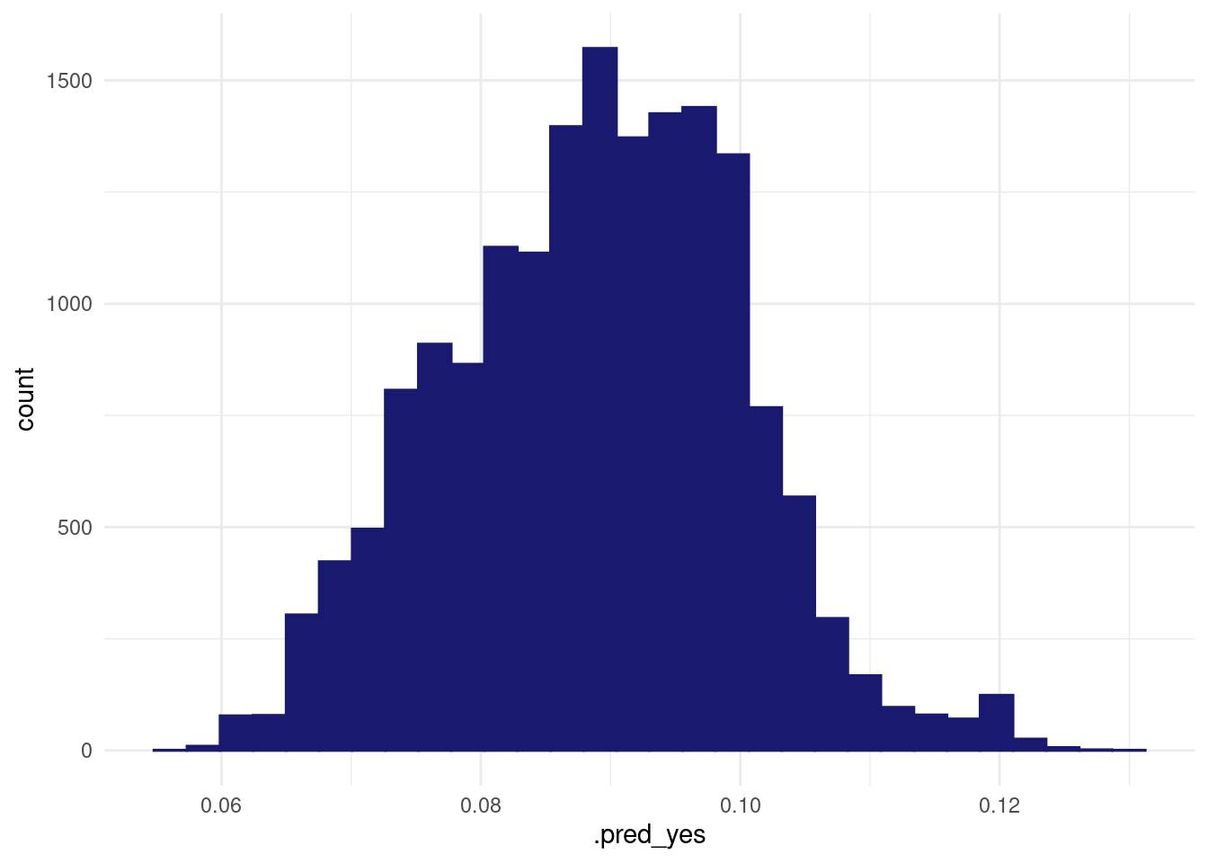
here’s how to check the metrics: () https://juliasilge.com/blog/nber-papers/)
collect_metrics(logistic_tuneable_xgb_wf_fit)## # A tibble: 2 × 4
## .metric .estimator .estimate .config
## <chr> <chr> <dbl> <chr>
## 1 accuracy binary 0.932 Preprocessor1_Model1
## 2 roc_auc binary 0.541 Preprocessor1_Model1collect_predictions(logistic_tuneable_xgb_wf_fit) %>%
conf_mat(has_claim_fct, .pred_class) %>%
autoplot()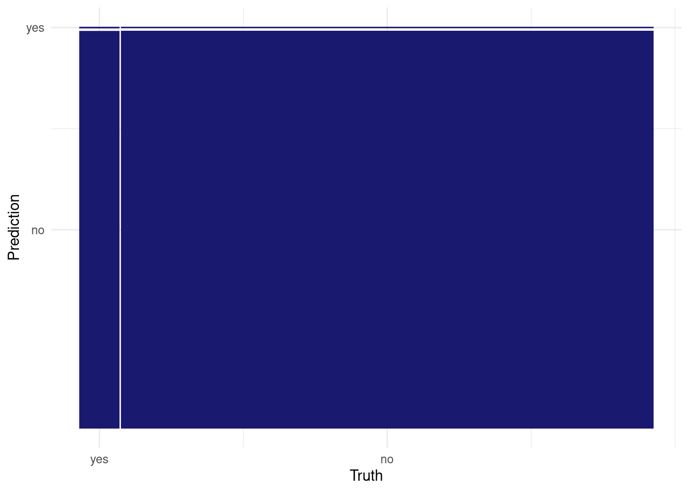
collect_predictions(logistic_tuneable_xgb_wf_fit) %>%
  roc_curve(truth = has_claim_fct, .pred_yes) %>%
  ggplot(aes(1 - specificity, sensitivity)) +
  geom_abline(slope = 1, color = "gray50", lty = 2, alpha = 0.8) +
  geom_path(size = 1.5, alpha = 0.7) +
  labs(color = NULL) +
  coord_fixed()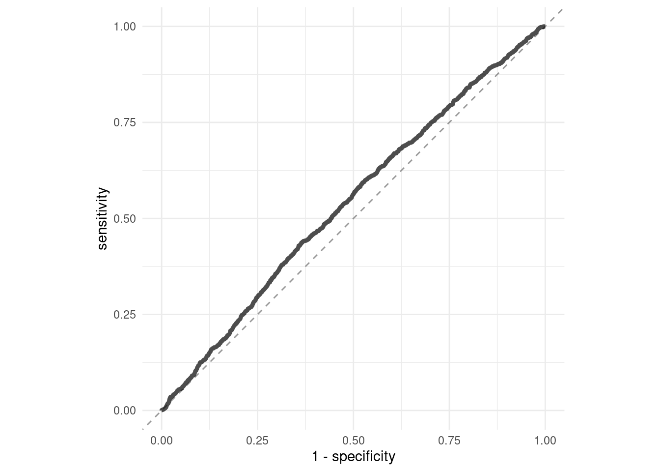
Logistic Regression with recipe pre-processor
ok, let’s use the option to pass a recipe instead of a formula to the workflow_set. This will allow us to do some feature engineering, like:
* imputing missing values (this doesnt happen in this dataset),
* create an “other” categorical values for factors levels that dont happen often (we’ll do that with area),
* replace high cardinality variables using using step_lencode_glm() (we’ll pretend that’s the case of veh_body, even though it only has 13 unique values.
my_recipe_with_imputation <- recipe(my_train ) %>%
  update_role(all_of(labels(terms(my_logistic_reg_formula))), new_role = "predictor") %>% # assign the role of predictor to right-side terms of my formula
  update_role(has_claim_fct, new_role= "outcome") %>%  ## was has_claim  in "my_recipe", but needs to be a factor for tidymodels
  update_role(exposure, new_role = "weight") %>%

  step_impute_median(all_numeric_predictors()) %>%  # impute median to missing numerical values
  step_impute_mode(all_nominal_predictors()) %>%  # impute mode to missing nominal values
  embed::step_lencode_glm(veh_body, outcome = vars(has_claim_fct)) %>% #  encode veh_body
  step_other(area, threshold = 0.10) %>%
  step_dummy(all_nominal_predictors())# %>%
#step_select(has_role(c("predictor", "outcome", "weight", "case_weights"))) # don't forger case_weights
we don’t actually need to prep/bake the recipe, but it’s interesting to check what is the output data.
prepped_recipe <- prep(my_recipe_with_imputation)
baked_train <- bake(prepped_recipe, my_train)
baked_train %>% glimpse()
## Rows: 50,893
## Columns: 18
## $ has_claim <int> 0, 0, 0, 0, 0, 0, 0, 0, 0, 1, 1, 0, 0, 0, 0, 0, 0, 0,…
## $ dollar_loss <dbl> 0.0000, 0.0000, 0.0000, 0.0000, 0.0000, 0.0000, 0.000…
## $ exposure <dbl> 0.64887064, 0.56947296, 0.85420945, 0.85420945, 0.555…
## $ veh_value <dbl> 1.03, 3.26, 2.01, 1.60, 1.47, 0.52, 1.38, 1.22, 1.00,…
## $ veh_body <dbl> -2.384210, -2.480687, -2.156805, -2.114655, -2.384210…
## $ veh_age <int> 2, 2, 3, 3, 2, 4, 2, 3, 2, 3, 3, 4, 3, 1, 4, 1, 2, 4,…
## $ agecat <int> 4, 2, 4, 4, 6, 3, 2, 4, 4, 4, 4, 2, 3, 1, 5, 1, 2, 3,…
## $ loss_cost <dbl> 0.0000, 0.0000, 0.0000, 0.0000, 0.0000, 0.0000, 0.000…
## $ policy_id <dbl> 2, 3, 6, 7, 7, 8, 10, 11, 12, 16, 16, 17, 18, 19, 19,…
## $ random <dbl> 0.937075413, 0.286139535, 0.519095949, 0.736588315, 0…
## $ has_claim_fct <fct> no, no, no, no, no, no, no, no, no, yes, yes, no, no,…
## $ exposure_weight <imp_wts> 0.64887064, 0.56947296, 0.85420945, 0.85420945, 0…
## $ policy_loss_cost <dbl> 0.0000, 0.0000, 0.0000, 0.0000, 0.0000, 0.0000, 0.000…
## $ gender_M <dbl> 0, 0, 1, 1, 1, 0, 1, 1, 0, 0, 1, 0, 0, 1, 1, 0, 0, 1,…
## $ area_B <dbl> 0, 0, 0, 0, 1, 0, 0, 0, 0, 0, 0, 0, 0, 0, 0, 1, 0, 0,…
## $ area_C <dbl> 0, 0, 1, 0, 0, 0, 0, 1, 1, 0, 1, 0, 1, 0, 1, 0, 0, 1,…
## $ area_D <dbl> 0, 0, 0, 0, 0, 0, 0, 0, 0, 0, 0, 1, 0, 0, 0, 0, 0, 0,…
## $ area_other <dbl> 0, 1, 0, 0, 0, 0, 0, 0, 0, 1, 0, 0, 0, 0, 0, 0, 0, 0,…as we can see, the dummies have been created and there are only 3 areas left (area_B, area_C, area_D), the other being bundled inside “area_other”. Also, the veh_body nominal variable has been replaced with a numeric variable with the following possible values.
baked_train %>% count(veh_body)## # A tibble: 13 × 2
## veh_body n
## <dbl> <int>
## 1 -2.64 54
## 2 -2.48 3448
## 3 -2.42 546
## 4 -2.38 14203
## 5 -2.35 16702
## 6 -2.32 1339
## 7 -2.26 12146
## 8 -2.16 1181
## 9 -2.11 568
## 10 -2.00 557
## 11 -1.66 93
## 12 -1.66 24
## 13 -0.965 32Looking at the original counds in the data, we understand that 0.9653894 (with n=32) is for “BUS” and 2.3842100 (with n=14203) is for UTE, the riskiest body type.
my_train %>% count(veh_body)## # A tibble: 13 × 2
## veh_body n
## <fct> <int>
## 1 BUS 32
## 2 CONVT 54
## 3 COUPE 557
## 4 HBACK 14203
## 5 HDTOP 1181
## 6 MCARA 93
## 7 MIBUS 546
## 8 PANVN 568
## 9 RDSTR 24
## 10 SEDAN 16702
## 11 STNWG 12146
## 12 TRUCK 1339
## 13 UTE 3448anyway, let’s create a workflow set with this recipe.
NOTE: I’M NOT SURE IF I CAN HAVE GAMs HERE BECAUSE THE FORMULA DEPENDS ON WHAT DUMMY THE RECIPE CREATED AND THIS MIGHT CHANGE FOR ALL RESAMPLES (given the use of step_other)
all_workflows5 <-
  workflow_set(
    preproc = list("recipe_with_imputation" = my_recipe_with_imputation ), # "recipe_with_feature_engineering"= my_recipe_with_imputation,
    models = list(
      logistic_glm = logistic_glm_spec,
      #logistic_gam = logistic_gam_spec#,
      logistic_xgboost = logistic_xgb_spec,
      logistic_tuneable_xgb = logistic_tuneable_xgb_spec
    ),
    case_weights = exposure_weight
  )
#
# all_workflows5 <- update_workflow_model(all_workflows5,
#                       i =  "recipe_with_imputation_logistic_gam",
#                       spec = logistic_gam_spec,
#                       formula = my_logistic_reg_formula)

# Workflows can take special arguments for the recipe (e.g. a blueprint) or a model (e.g. a special formula). However, when creating a workflow set, there is no way to specify these extra components. update_workflow_model() and update_workflow_recipe() allow users to set these values after the workflow set is initially created. They are analogous to workflows::add_model() or workflows::add_recipe().

all_workflows6 <-
  all_workflows5 %>%
  workflow_map(resamples = train_resamples,
               fn = "tune_grid",
               verbose = TRUE)
autoplot(all_workflows6, metric="roc_auc")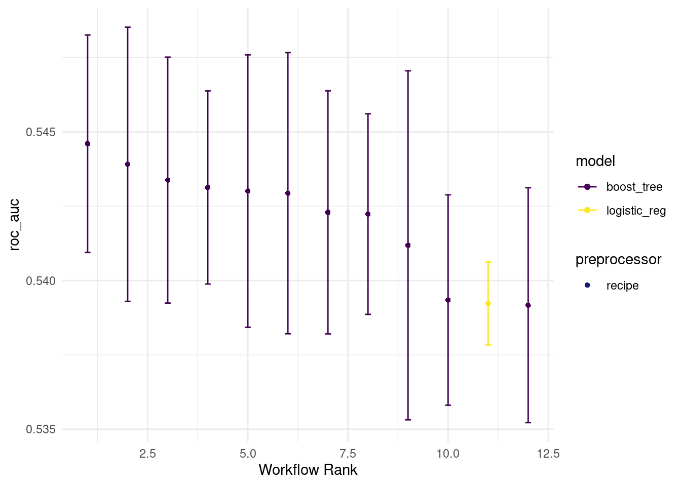
rank_results(all_workflows6, rank_metric = "roc_auc")## # A tibble: 24 × 9
## wflow_id .config .metric mean std_err n preprocessor model rank
## <chr> <chr> <chr> <dbl> <dbl> <int> <chr> <chr> <int>
## 1 recipe_with_imp… Prepro… accura… 0.932 0.00133 5 recipe boos… 1
## 2 recipe_with_imp… Prepro… roc_auc 0.545 0.00222 5 recipe boos… 1
## 3 recipe_with_imp… Prepro… accura… 0.932 0.00133 5 recipe boos… 2
## 4 recipe_with_imp… Prepro… roc_auc 0.544 0.00280 5 recipe boos… 2
## 5 recipe_with_imp… Prepro… accura… 0.932 0.00133 5 recipe boos… 3
## 6 recipe_with_imp… Prepro… roc_auc 0.543 0.00251 5 recipe boos… 3
## 7 recipe_with_imp… Prepro… accura… 0.932 0.00133 5 recipe boos… 4
## 8 recipe_with_imp… Prepro… roc_auc 0.543 0.00198 5 recipe boos… 4
## 9 recipe_with_imp… Prepro… accura… 0.932 0.00133 5 recipe boos… 5
## 10 recipe_with_imp… Prepro… roc_auc 0.543 0.00279 5 recipe boos… 5
## # ℹ 14 more rowslet’s fit the best model on the ful ldata set and check how it performs on the test set :
best_workflow_fit <- all_workflows6 %>%
  extract_workflow("recipe_with_imputation_logistic_tuneable_xgb") %>%
  finalize_workflow(select_best(all_workflows6 %>%
                                  extract_workflow_set_result("recipe_with_imputation_logistic_tuneable_xgb"), metric = "roc_auc")
  ) %>%
  last_fit(split= my_split)

best_workflow_fit %>%
  extract_fit_engine() %>%
  vip(num_features=20)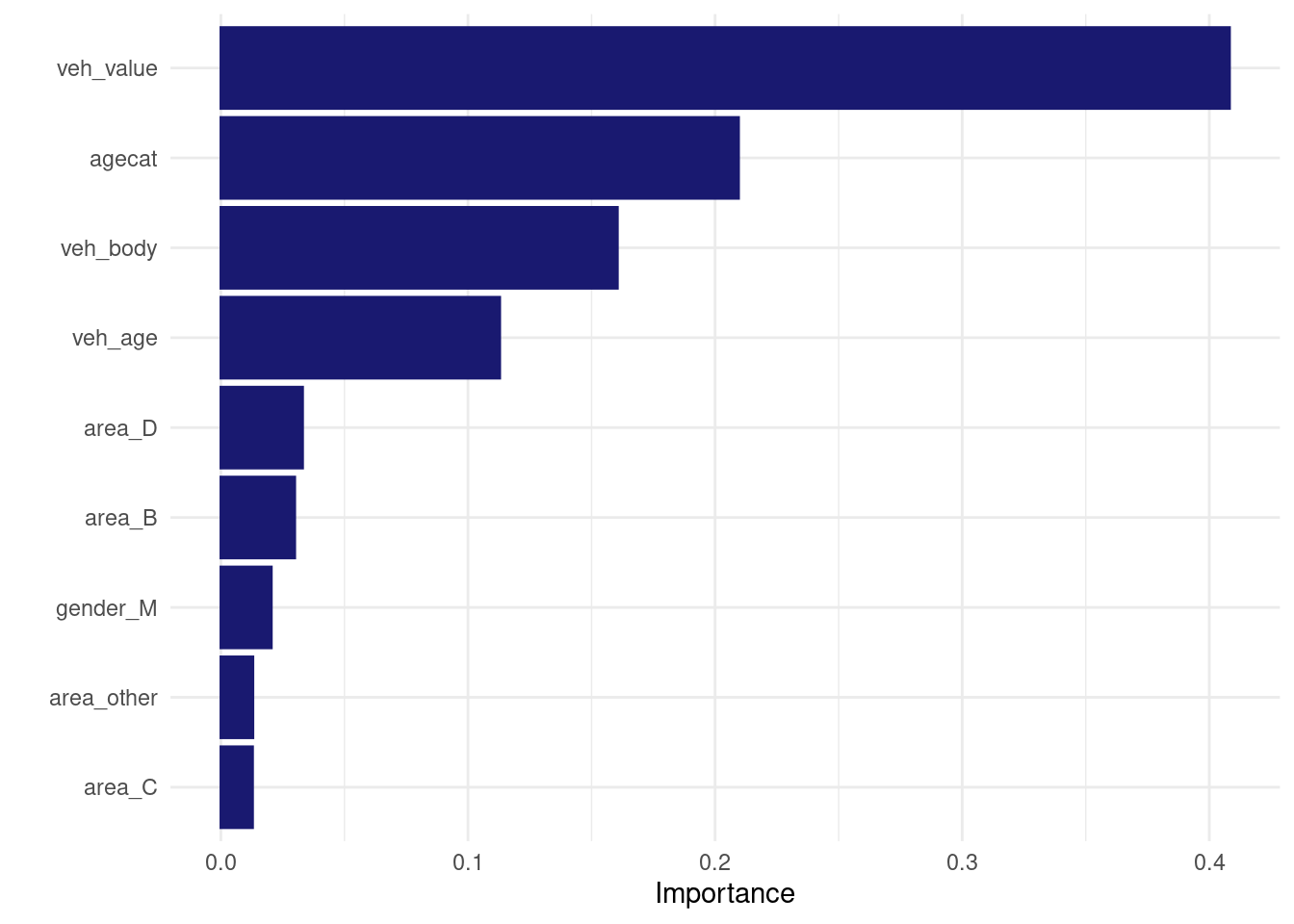
Tweedie regression
alright that was fun, let’s try to model the weedie.
my_loss_cost_formula <- as.formula("loss_cost ~ veh_value + veh_body + veh_age + gender + area + agecat")Estimate tweedie “p” parameter
We first need to estimate the tweedie index parameter p. I will do it only once on the full training data set. There will be some data leak when estimating the resamples, but I’m not sure how I could estimate it for each resamples.
We use tweedie.profile() to estimate the p parameter. If the tweedie.profile() function fails to converge, we can try switching the method to “saddeploint” or “interpolation” (as per ?tweedie.profile).
out <- tweedie::tweedie.profile(
  my_loss_cost_formula,
  data = my_train,
  p.vec = seq(1.05, 1.95, by=0.05),
  weights= my_train$exposure,
  link.power = 0,
  do.smooth= TRUE,
  do.plot = TRUE)
## 1.05 1.1 1.15 1.2 1.25 1.3 1.35 1.4 1.45 1.5 1.55 1.6 1.65 1.7 1.75 1.8 1.85 1.9 1.95
## ...................Done.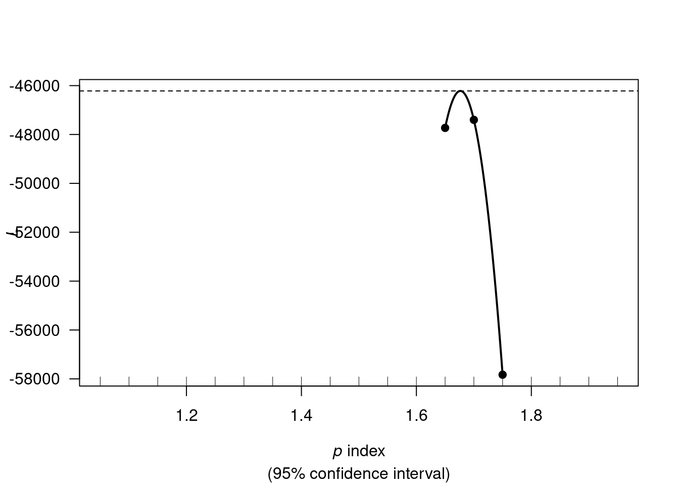
out## $y
## [1] -47730.79 -47506.76 -47300.66 -47112.47 -46942.21 -46789.86 -46655.44
## [8] -46538.95 -46440.37 -46359.71 -46296.98 -46252.17 -46225.28 -46216.32
## [15] -46225.27 -46252.15 -46296.94 -46359.67 -46440.31 -46538.87 -46655.36
## [22] -46789.76 -46942.09 -47112.35 -47300.52 -47506.61 -47730.63 -47972.57
## [29] -48232.43 -48510.21 -48805.92 -49119.54 -49451.09 -49800.56 -50167.95
## [36] -50553.27 -50956.50 -51377.66 -51816.74 -52273.74 -52748.66 -53241.51
## [43] -53752.27 -54280.96 -54827.57 -55392.10 -55974.56 -56574.93 -57193.23
## [50] -57829.45
##
## $x
## [1] 1.650000 1.652041 1.654082 1.656122 1.658163 1.660204 1.662245 1.664286
## [9] 1.666327 1.668367 1.670408 1.672449 1.674490 1.676531 1.678571 1.680612
## [17] 1.682653 1.684694 1.686735 1.688776 1.690816 1.692857 1.694898 1.696939
## [25] 1.698980 1.701020 1.703061 1.705102 1.707143 1.709184 1.711224 1.713265
## [33] 1.715306 1.717347 1.719388 1.721429 1.723469 1.725510 1.727551 1.729592
## [41] 1.731633 1.733673 1.735714 1.737755 1.739796 1.741837 1.743878 1.745918
## [49] 1.747959 1.750000
##
## $ht
## [1] -46218.24
##
## $L
## [1] NaN NaN NaN NaN -Inf -Inf -Inf
## [8] -Inf -Inf -Inf -Inf -Inf -47730.79 -47401.33
## [15] -57829.45 NA NA NA NA
##
## $p
## [1] 1.05 1.10 1.15 1.20 1.25 1.30 1.35 1.40 1.45 1.50 1.55 1.60 1.65 1.70 1.75
## [16] 1.80 1.85 1.90 1.95
##
## $p.max
## [1] 1.676531
##
## $L.max
## [1] -46216.32
##
## $phi
## [1] 15721.8783 14176.4100 7900.2438 4402.6561 3969.8736 2212.3358
## [7] 1232.8935 1111.7004 619.5304 558.6312 311.3155 280.7140
## [13] 498.4586 412.0971 3468.7345 NA NA NA
## [19] NA
##
## $phi.max
## [1] 449.5171
##
## $ci
## [1] 2.300698 2.300698
##
## $method
## [1] "inversion"
##
## $phi.method
## [1] "mle"Our estimate for the tweedie p parameter is out$p.max.
FUN #3 !!! For some reason, when I dont round my_p_max (or I keep more than 3 digits), my “direct” tweedie xgboost has slightly different results than the tidymodels xgboost.
my_p_max <- round(out$p.max, digits = 2)
my_p_max
## [1] 1.68Reproducing “non-tidymodels” specs in tidymodels
GLM weighted
direct call to glm() with tweedie family:
tweedie_fit <-
  glm(formula =  my_loss_cost_formula,
      family=tweedie(var.power=my_p_max, link.power=0),
      weights = exposure,
      data = my_train)

tweedie_fit %>% tidy()
## # A tibble: 22 × 5
## term estimate std.error statistic p.value
## <chr> <dbl> <dbl> <dbl> <dbl>
## 1 (Intercept) 5.81 2.56 2.27 0.0231
## 2 veh_value 0.0624 0.0939 0.664 0.507
## 3 veh_bodyCONVT -2.32 4.21 -0.550 0.582
## 4 veh_bodyCOUPE 0.441 2.60 0.169 0.866
## 5 veh_bodyHBACK -0.123 2.52 -0.0490 0.961
## 6 veh_bodyHDTOP 0.110 2.55 0.0430 0.966
## 7 veh_bodyMCARA -0.758 3.19 -0.238 0.812
## 8 veh_bodyMIBUS -0.111 2.61 -0.0425 0.966
## 9 veh_bodyPANVN -0.192 2.59 -0.0741 0.941
## 10 veh_bodyRDSTR -0.927 4.74 -0.196 0.845
## # ℹ 12 more rowstidymodels call glm regression with tweedie family:
tweedie_glm_spec <-
  parsnip::linear_reg(mode = "regression") %>%
  parsnip::set_engine("glm", family=tweedie(var.power=my_p_max, link.power=0))


tweedie_glm_wf <-   workflow() %>%
  add_case_weights(exposure_weight) %>%
  add_formula(my_loss_cost_formula) %>%
  add_model(tweedie_glm_spec)

tweedie_glm_wf_fit <-  tweedie_glm_wf %>%
  fit(data = my_train)

tweedie_glm_wf_fit %>%  tidy()
## # A tibble: 22 × 5
## term estimate std.error statistic p.value
## <chr> <dbl> <dbl> <dbl> <dbl>
## 1 (Intercept) 5.81 2.56 2.27 0.0231
## 2 veh_value 0.0624 0.0939 0.664 0.507
## 3 veh_bodyCONVT -2.32 4.21 -0.550 0.582
## 4 veh_bodyCOUPE 0.441 2.60 0.169 0.866
## 5 veh_bodyHBACK -0.123 2.52 -0.0490 0.961
## 6 veh_bodyHDTOP 0.110 2.55 0.0430 0.966
## 7 veh_bodyMCARA -0.758 3.19 -0.238 0.812
## 8 veh_bodyMIBUS -0.111 2.61 -0.0425 0.966
## 9 veh_bodyPANVN -0.192 2.59 -0.0741 0.941
## 10 veh_bodyRDSTR -0.927 4.74 -0.196 0.845
## # ℹ 12 more rowsit’s identical, yes!
GAM (with splines) weighted
my_loss_cost_spline_formula <- as.formula('loss_cost ~ s(veh_value, bs= "tp") + veh_body + veh_age + gender + area + agecat')tweedie_gam_spec <-
gen_additive_mod() %>%
set_engine('mgcv', method= "REML", family = Tweedie(p = my_p_max, link = "log")) %>%
set_mode('regression')
tweedie_gam_wf <- workflow() %>%
add_model(tweedie_gam_spec, formula = my_loss_cost_spline_formula) %>% # need to add formula twice, and in add_formula
add_formula(my_loss_cost_formula) %>%
add_case_weights(exposure_weight)
tweedie_gam_wf_fit <- tweedie_gam_wf%>%
fit(data = my_train )
tweedie_gam_wf_fit %>% tidy(parametric = TRUE)## # A tibble: 21 × 5
## term estimate std.error statistic p.value
## <chr> <dbl> <dbl> <dbl> <dbl>
## 1 (Intercept) 5.92 1.23 4.83 0.00000136
## 2 veh_bodyCONVT -2.32 2.03 -1.14 0.254
## 3 veh_bodyCOUPE 0.441 1.26 0.351 0.726
## 4 veh_bodyHBACK -0.123 1.22 -0.101 0.919
## 5 veh_bodyHDTOP 0.110 1.23 0.0890 0.929
## 6 veh_bodyMCARA -0.759 1.54 -0.493 0.622
## 7 veh_bodyMIBUS -0.112 1.26 -0.0884 0.930
## 8 veh_bodyPANVN -0.192 1.25 -0.153 0.878
## 9 veh_bodyRDSTR -0.928 2.29 -0.406 0.685
## 10 veh_bodySEDAN -0.138 1.21 -0.113 0.910
## # ℹ 11 more rowssame result if I do it directly using mgcv::gam?
mgcv::gam(
  formula = my_loss_cost_spline_formula,
  data = my_train,
  weights = exposure,
  family = Tweedie(p = my_p_max, link = "log"),
  method="REML") %>%
  broom::tidy(parametric= TRUE)
## # A tibble: 21 × 5
## term estimate std.error statistic p.value
## <chr> <dbl> <dbl> <dbl> <dbl>
## 1 (Intercept) 5.92 1.23 4.83 0.00000136
## 2 veh_bodyCONVT -2.32 2.03 -1.14 0.254
## 3 veh_bodyCOUPE 0.441 1.26 0.351 0.726
## 4 veh_bodyHBACK -0.123 1.22 -0.101 0.919
## 5 veh_bodyHDTOP 0.110 1.23 0.0890 0.929
## 6 veh_bodyMCARA -0.759 1.54 -0.493 0.622
## 7 veh_bodyMIBUS -0.112 1.26 -0.0884 0.930
## 8 veh_bodyPANVN -0.192 1.25 -0.153 0.878
## 9 veh_bodyRDSTR -0.928 2.29 -0.406 0.685
## 10 veh_bodySEDAN -0.138 1.21 -0.113 0.910
## # ℹ 11 more rowsYES!! ESTI QUE JE SUIS BON AHAH!
XGBoost weighted
Here’s how I could train an xgboost outside parsnip:
NOTE: I need to one-hot encode dummy variables to match what {tidymodels} do.
my_tweedie_recipe <- recipe(my_train ) %>%
  update_role(all_of(labels(terms(my_loss_cost_formula))), new_role = "predictor") %>%
  update_role(loss_cost, new_role= "outcome") %>%
  update_role(exposure, new_role = "weight") %>%
  step_dummy(all_nominal_predictors(), one_hot = TRUE) %>% ## APPARENTLY tidymodels use one_hot = TRUE because their model has 24 features. when I dont set one_hot  I only have 21 features.
  step_select(has_role(c("predictor", "outcome", "weight")))

prepped_tweedie_recipe <- prep(my_tweedie_recipe)
baked_train <- bake(prepped_tweedie_recipe, my_train)
baked_test <- bake(prepped_tweedie_recipe, my_test)

my_params <- list(
  eta = 0.1,
  max_depth = 3,
  gamma = 0,
  colsample_bytree = 1,
  colsample_bynode = 1,
  min_child_weight = 50,
  subsample = 1,
  nthread = 1)

xgtrain <- xgboost::xgb.DMatrix(
  data = as.matrix(baked_train %>% select(-loss_cost, -exposure)),
  label = baked_train$loss_cost,
  weight = baked_train$exposure
)

xgtest <- xgboost::xgb.DMatrix(
  data = as.matrix(baked_test %>% select(-loss_cost, -exposure)),
  label = baked_test$loss_cost,
  weight = baked_test$exposure
)

set.seed(456)
direct_xgb_tweedie_fit <- xgboost::xgb.train(
  data = xgtrain,
  params = my_params,
  nrounds = 200,
  objective = "reg:tweedie",
  eval_metric=paste0("tweedie-nloglik@",my_p_max),
  tweedie_variance_power = my_p_max
)
vip::vip(direct_xgb_tweedie_fit, num_features = 30L)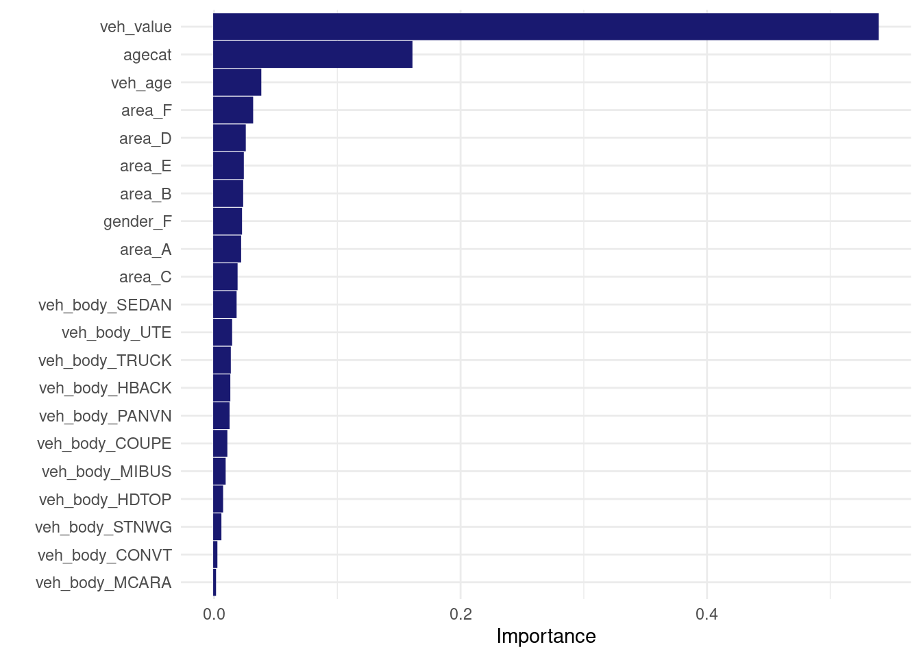
Here’s how I would train the same model in tidymodels:
tweedie_xgb_spec <-
  boost_tree(
    tree_depth = 3,
    trees= 200,
    learn_rate = 0.1,
    min_n = 50,
    loss_reduction = 0,
    sample_size = 1.0,
    stop_iter = NULL
  ) %>%
  set_engine('xgboost', nthread = 1,
             objective = "reg:tweedie",
             eval_metric=paste0("tweedie-nloglik@",my_p_max),
             tweedie_variance_power = my_p_max) %>% ##https://www.kaggle.com/code/olehmezhenskyi/tweedie-xgboost
  set_mode('regression')


tweedie_xgb_wf <- workflow() %>%
  add_model(tweedie_xgb_spec) %>%
  add_formula(my_loss_cost_formula) %>%
  add_case_weights(exposure_weight)

set.seed(456)
tweedie_xgb_wf_fit <-  tweedie_xgb_wf%>%
  fit(data = my_train )


tweedie_xgb_wf_fit %>% extract_fit_engine() %>% vip::vip(num_features = 30L)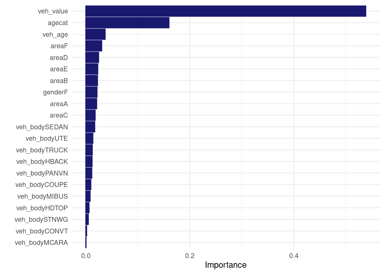
let’s compare them:
Same predictions for the first.. 6 digits?
pred_tidy <- predict(tweedie_xgb_wf_fit, new_data = my_test)
pred_direct <- predict(direct_xgb_tweedie_fit, newdata = xgtest)
z <- pred_tidy %>% rename(pred_tidy = .pred) %>%  add_column(pred_direct) %>%
  mutate(diff_percent = (pred_tidy-pred_direct)/pred_tidy)
z %>% ggplot(aes(x= pred_tidy, y = pred_direct)) +
  geom_point(alpha = 0.05) +
  geom_smooth() +
  coord_equal()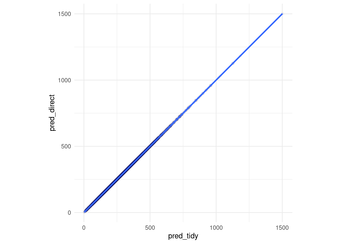
z %>% select(diff_percent) %>% skimr::skim()| Name | Piped data |
| Number of rows | 16963 |
| Number of columns | 1 |
| _______________________ | |
| Column type frequency: | |
| numeric | 1 |
| ________________________ | |
| Group variables | None |
Variable type: numeric
| skim_variable | n_missing | complete_rate | mean | sd | p0 | p25 | p50 | p75 | p100 | hist |
|---|---|---|---|---|---|---|---|---|---|---|
| diff_percent | 0 | 1 | 0 | 0 | 0 | 0 | 0 | 0 | 0 | ▁▁▇▁▁ |
Identical first tree? tidymodels xgboost model tree #1:
xgb.plot.tree(model = tweedie_xgb_wf_fit %>% extract_fit_engine(), trees = 1)direct xgboost model tree #1:
xgb.plot.tree(model = direct_xgb_tweedie_fit, trees = 1)same parameters?
tidymodels parameters:
tweedie_xgb_wf_fit %>% extract_fit_engine()## ##### xgb.Booster
## raw: 226.2 Kb
## call:
## xgboost::xgb.train(params = list(eta = 0.1, max_depth = 3, gamma = 0,
## colsample_bytree = 1, colsample_bynode = 1, min_child_weight = 50,
## subsample = 1), data = x$data, nrounds = 200, watchlist = x$watchlist,
## verbose = 0, nthread = 1, objective = "reg:tweedie", eval_metric = "tweedie-nloglik@1.68",
## tweedie_variance_power = 1.68)
## params (as set within xgb.train):
## eta = "0.1", max_depth = "3", gamma = "0", colsample_bytree = "1", colsample_bynode = "1", min_child_weight = "50", subsample = "1", nthread = "1", objective = "reg:tweedie", eval_metric = "tweedie-nloglik@1.68", tweedie_variance_power = "1.68", validate_parameters = "TRUE"
## xgb.attributes:
## niter
## callbacks:
## cb.evaluation.log()
## # of features: 24
## niter: 200
## nfeatures : 24
## evaluation_log:
## iter training_tweedie_nloglik@1.68
## 1 625.66655
## 2 566.66643
## ---
## 199 26.83899
## 200 26.83779direct fit parameters:
direct_xgb_tweedie_fit## ##### xgb.Booster
## raw: 226.2 Kb
## call:
## xgboost::xgb.train(params = my_params, data = xgtrain, nrounds = 200,
## objective = "reg:tweedie", eval_metric = paste0("tweedie-nloglik@",
## my_p_max), tweedie_variance_power = my_p_max)
## params (as set within xgb.train):
## eta = "0.1", max_depth = "3", gamma = "0", colsample_bytree = "1", colsample_bynode = "1", min_child_weight = "50", subsample = "1", nthread = "1", objective = "reg:tweedie", eval_metric = "tweedie-nloglik@1.68", tweedie_variance_power = "1.68", validate_parameters = "TRUE"
## xgb.attributes:
## niter
## callbacks:
## cb.print.evaluation(period = print_every_n)
## # of features: 24
## niter: 200
## nfeatures : 24TODO: Poisson regression
Reproducing “non-tidymodels” specs in tidymodels
GLM weighted
GAM (with splines) weighted
xgboost weighted
TODO: Gamma regression
stackoverflow adding gamma to glm regression: https://stackoverflow.com/questions/66024469/glm-family-using-tidymodels
## Reproducing “non-tidymodels” specs in tidymodels
### GLM weighted
### GAM (with splines) weighted
### xgboost weighted
resources
- tidy modelling with r book https://www.tmwr.org/resampling
- all of juliasilge’s blog posts juliasilge.com
- just stumbled on this website by taylor dunn as I put the finishing touch to this post (damn https://bookdown.org/taylordunn/islr-tidy-1655226885741/moving-beyond-linearity.html)